Efficient Zero-Knowledge Arguments for Arithmetic Circuits in the Discrete Log Setting学习笔记-程序员宅基地
技术标签: 零知识证明
1. 引言
Bootle和Groth等人2016年论文《Efficient Zero-Knowledge Arguments for Arithmetic Circuits in the Discrete Log Setting》。
在本论文中,主要为 (只有加法门和乘法门的) arithmetic circcuit satisfiability 提供了一种零知识证明算法,具有的communication complexity为 O ( log n ) O(\log n) O(logn),其中 n n n为circuit size;具有的round complexity也为 O ( log n ) O(\log n) O(logn)。且对于所有gates均为 2 fan-in的arithmetic circuit,Prover和Verifier的computation complexity均为 O ( n ) O(n) O(n)。该算法无需trusted setup,仅需基于discrete logarithm assumption in prime order groups即可。
在该零知识证明算法中,核心内容为:
- inner product 零知识证明算法。
该inner product 零知识证明算法,具有的communication complexity为 O ( log n ) O(\log n) O(logn),round complexity为 O ( log n ) O(\log n) O(logn),Prover和Verifier的computation complexity均为 O ( n ) O(n) O(n)。
除此之外,还提供了一种polynomial commitment算法,用于reveal the evaluation at an arbitrary point in a verifiable manner。使用该polynomial commitment算法,可将Groth 2009年论文《Linear Algebra with Sub-linear Zero-Knowledge Arguments》中的constant round arithmetic circuit 零知识证明算法的communication complexity 由 O ( n ) O(\sqrt{n}) O(n)进一步优化降低为 O ( log n ) O(\log n) O(logn)。(可参见博客 Linear Algebra with Sub-linear Zero-Knowledge Arguments学习笔记)
零知识证明算法可广泛用于authentication protocol, multi-parity computation, encryption primitives, electronic voting systems和verifiable computation protocols。
零知识证明算法应具有如下属性:
- Completeness:A prover with a witness w w w for u ∈ L u\in L u∈L can convince the verifier of this fact.
- Soundness:A prover cannot convince a verifier when u ∉ L u\notin L u∈/L.
- Zero-knowledge:The interaction should not reveal anything to the verifier except that u ∈ L u\in L u∈L. In particular, it should not reveal the prover’s witness w w w.
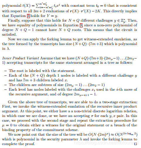
[Gro09b] Groth 2009年论文《Linear Algebra with Sub-linear Zero-Knowledge Arguments》中各算法性能表现为:
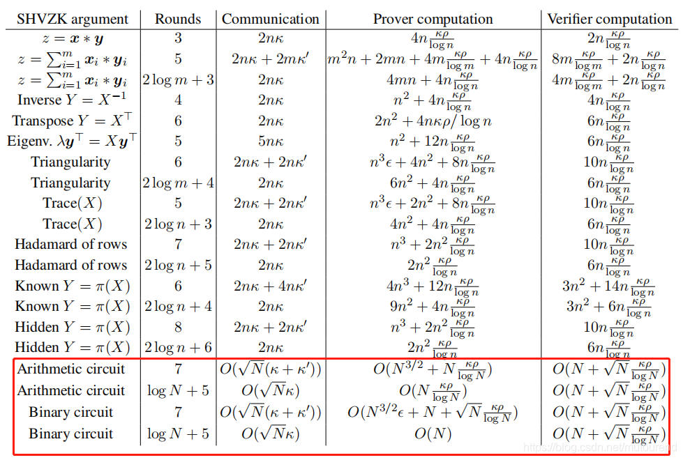
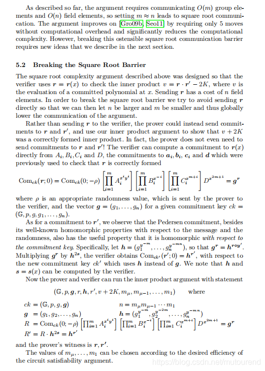
上图Arithmetic circuit constant round 零知识证明算法中,需要7 moves,具有square root communication complexity in the total number of gates。在该算法中,Prover需commits to all the wires using homomorphic multicommitments, 对于加法门可利用同态属性来verify,对于乘法门可利用product argument来verify。
本文在[Gro09b]算法的基础上,分为两大步来改进:
1)首先实现5 moves,communication complexity为square root的argument:
- 避免使用[Gro09b]中的generic reductions to linear algebra statements,可由7 moves降为5 moves;
- 通过同时处理一系列的Hadamard products和linear relations,可去除argument中加法门的communication cost,comminication complexity 由 O ( n a d d + n m u l ) O(\sqrt{n_{add}+n_{mul}}) O(nadd+nmul)降为 O ( n m u l ) O(\sqrt{n_{mul}}) O(nmul)(其中 n a d d + n m u l n_{add}+n_{mul} nadd+nmul代表total number of gates,而 n m u l n_{mul} nmul为multiplication gates的数量。)。
- 同时还提出了一种polynomial commitment 零知识证明算法,其communication complexity为 O ( d ) O(\sqrt{d}) O(d),其中 d d d为polynomial degree。
2)其次,在1)的基础上,进一步压缩communication complexity:
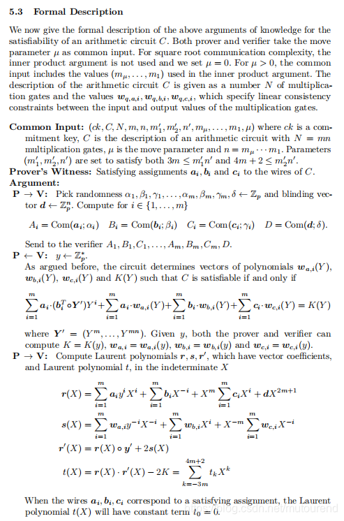
- 在1)算法中,仍然具有communication complexity O ( n m u l ) O(\sqrt{n_{mul}}) O(nmul)。原因是在第一轮Prover需要commit to all circuit wires using 3 m 3m 3m commitments to n n n elements each,其中 m n = N mn=N mn=N 为multiplication gate数量的上线。而在最后一轮当收到challenge后,Prover open one commitment that can be constructed from the previous ones and the challenge。当设置 m ≈ n m\approx n m≈n时,最小communication complexity即为 O ( N ) O(\sqrt{N}) O(N)。
本文将最后一轮的opening step替换为了an argument of knowledge of the opening values,利用Pedersen multicommitments的同态属性,将该argument实现为an argument of knowledge of openings of two homomorphic commitments,satisfying an inner product relation。该inner product argument通过借助递归方法,其communication complexity为 O ( log n ) O(\log n) O(logn),其中 n n n为vector size。借助该inner product argument,其最终实现的arithmetic circuit satisfiability argument的communication也为logarithmic。
将本文最终实现的5 moves, O ( log n ) O(\log n) O(logn) communication argument算法与Pinocchio算法([PHGR13] 2013年Parno等人论文 Pinocchio: Nearly practical verifiable computation)进行对比:(Pinocchio为使用的verifiable computation scheme,允许constrained client将a function的computation 外包给 a powerful worker,同时能高效验证该worker输出的function运算结果是否正确。Pinocchio采用quadratic arithmetic programs,为arithmetic circuits的generalisation,可以实现比本地直接计算更快的function verification。)
- 本文算法的verification虽然不够快,但是在基于更简单的assumption的基础上,具有更快的prover computation。
1.1 相关研究工作
-
Goldwasser等人在1989(1985)年论文《The knowledge complexity of interactive proofs》中首次提出了Zero-knowledge proofs概念。
注意区分:
– zero-knowledge proof:具有statistical soundness。proof仅能有computational zero-knowledge。
– zero-knowledge argument:具有computational soundness。而argument可能有perfect zero-knowledge。 -
Brassard等人1988年论文《Minimum disclosure proofs of knowledge》中指出 all languages in NP have zero-knowledge arguments with perfect zero-knowledge。
-
Goldreich等人1991年论文《Proofs that yield nothing but their validity or all languages in NP have zero-knowledge proof systems》中指出 all languages in NP have zero-knowledge proofs。
-
Gentry等人2014年论文《Using fully homomorphic hybrid encryption to minimize non-interative zero-knowledge proofs》中采用全同态加密算法来构建 zero-knowledge proofs,其communication complexity与witness size相当。通常地,proofs的communication不会小于witness size,除非 surprising results about the complexity of solving SAT instances hold(参见论文[GH98][GVW02])。
-
Kilian在1992年论文《 A note on efficient zero-knowledge proofs and arguments》中指出,与 zero-knowledge proofs不同,若只实现 zero-knowledge arguments的话,可以具有很低的communication complexity。Kilian的构建依赖于 PCP theorem,无法生成实用的scheme。
-
Schnorr 1991年论文《Efficient signature generation by smart cards》和Guilou等人1988年论文《 A practical zero-knowledge protocol fitted to security microprocessor minimizing both trasmission and memory》给出了早期的实用的zero-knowledge arguments for concrete number theoretic problems例子。基于Schnorr protocol,可扩展出很多基于discrete logarithms assumption的zero-knowledge arguments。
-
Cramer等人1998年论文《Zero-knowledge proofs for finite field arithmetic; or: Can zero-knowledge be for free?》中给出了基于arithmetic circuit satisfiability的zero-knowledge argument算法,该算法具有linear communication complexity。
-
截至目前(2016年),基于discrete logarithm assumption 构建的arithmetic circuit zero-knowledge argument 最高效的算法有 Groth 2009年论文《Linear Algebra with Sub-linear Zero-Knowledge Arguments》中算法和Seo 2011年论文《Round-efficient sub-linear zero-knowledge arguments for linear algebra》中算法,二者均具有constant move,communication complexity为square root of the circuit size。 O ( N ) O(\sqrt{N}) O(N)
-
若不基于 discrete logarithm assumption,而采用 pairing-based cryptography,Groth 2009年论文《Efficient zero-knowledge arguments from two-tiered homomorphic commitments》中生成的arithmetic circuit zero-knowledge argument 具有 cubic root communication complexity。 O ( N 3 ) O(\sqrt[3]{N}) O(3N)
-
目前基于 specific languages构建的具有logarithmic communication complexity的算法有:(这些都是针对特定类型的statements——具有low circuit depth,且这些算法无法推广至任意的NP languages。)
– 2013年Bayer和Groth 论文《Zero-knowledge argument for polynomial evaluation with application to blacklists》中指出,one can prove that a polynomial evaluated at a secret committed value gives a certain output with a logarithmic communication complexity。【注意普通的polynomial commitment,其evaluate的点是公开的,而此处是secret的。】
– 2014年Groth和Kohlweiss 论文《One-out-of-many proofs: Or how to leak a secret and spend a coin》中指出,one out of N N N commitments contain 0 with logarithmic communication complexity。 -
以下系列的研究均是基于pairing-based cryptography构建的succinct non-interactive arguments (SNARGs),其argument具有 a constant number of group elements,但是它们都依赖于 a common reference string (with a special structure) and non-falsifiable knowledge extractor assumption:
– Groth 2010年论文《Short pairing-based non-interactive zero-knowledge arguments》
– Lipmaa 2012年论文《Progression-free sets and sublinear pairing-based non-interactive zero-knowledge arguments》
– Bitansky等人2012年论文《From extractable collision resistance to succinct non-interactive arguments of knowledge, and back again》
– Gennaro等人2013年论文《Quadratic span programs and succinct NIZKs without PCPs》
– Bitansky等人2013年论文《Recursive composition and bootstrapping for SNARKS and proof-carrying data》
– Parno等人2013年论文《 Pinocchio: Nearly practical verifiable computation》
– Ben-Sasson等人2013年论文《SNARKs for C: verifying program executions succinctly and in Zero Knowledge》
– Ben-Sasson等人2014年论文《Succinct non-interactive zero knowledge for a von neumann architecture》
– Groth和Kohlweiss 2014年论文《One-out-of-many proofs: Or how to leak a secret and spend a coin》 -
本文构建的argument仅基于discrete logartihm assumption,且使用与 circuit无关的 small common reference string。
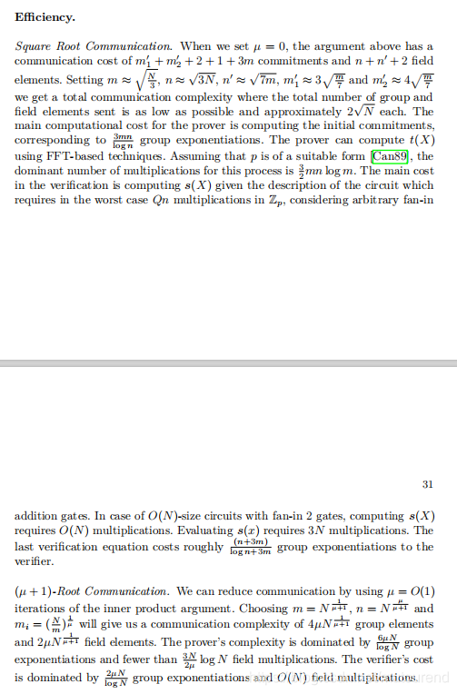
以下为对当前最高效的基于discrete logarithm assumption的zero-knowledge arguments的性能对比:
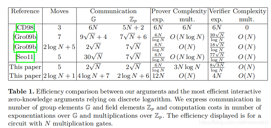
由上图可知:
- 同样是5 moves, 本文算法所需要的computation低于[Seo11]算法;
- 当使用logarithmic number of moves时,本文采用了与2012年论文《Efficient zero-knowledge argument for correctness of a shuffle》类似的reduction,在不增加其它开销的情况下,可大幅降低communication cost。与2012年论文《Efficient zero-knowledge argument for correctness of a shuffle》中使用reduction来降低computation不同,本文用来降低communication。(参见博客 Efficient Zero-Knowledge Argument for Correctness of a Shuffle学习笔记(1))
1.2 polynomial commitment
-
Kate等人2010年论文《Constant-size commitments to polynomials and their applications》中提供了a protocol to commit to polynomial and then evaluate it at a given point in a verifiable way。该算法仅需a constant number of commitments,但是其security依赖于pairing assumption。
-
本文构建的polynomial commitment 具有 square root communication complexity,但是完全基于discrete logarithm assumption。
1.3 相关定义
A multi-exponentiation of size n n n can be computed at a cost of roughly n log n \frac{n}{\log n} lognn single group exponentiations using the multi-exponentiation techniques of [Lim00, M¨ol01, MR08]。

- Pedersen Commitment定义:
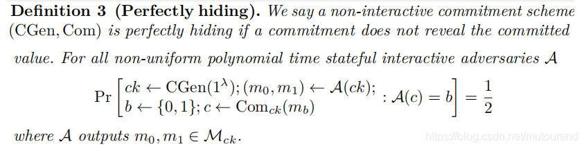
Breaking the binding property of Pedersen commitments corresponds to breaking the discrete logarithm assumption.
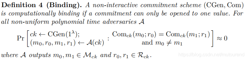
Pedersen commitment具有加法同态属性:
C o m c k ( m 0 ; r 0 ) ⋅ C o m c k ( m 1 ; r 1 ) = C o m c k ( m 0 + m 1 ; r 0 + r 1 ) Com_{ck}(m_0;r_0)\cdot Com_{ck}(m_1;r_1)=Com_{ck}(m_0+m_1;r_0+r_1) Comck(m0;r0)⋅Comck(m1;r1)=Comck(m0+m1;r0+r1)
Pedersen multicommitment指:
C o m c k ( m 1 , ⋯ , m n ; r ) = g r ∏ i = 1 n g i m i Com_{ck}(m_1,\cdots,m_n;r)=g^r\prod_{i=1}^{n}g_i^{m_i} Comck(m1,⋯,mn;r)=gr∏i=1ngimi
-
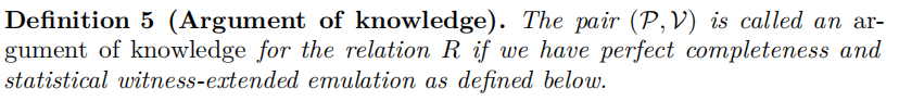
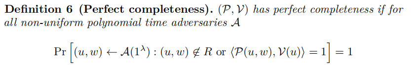
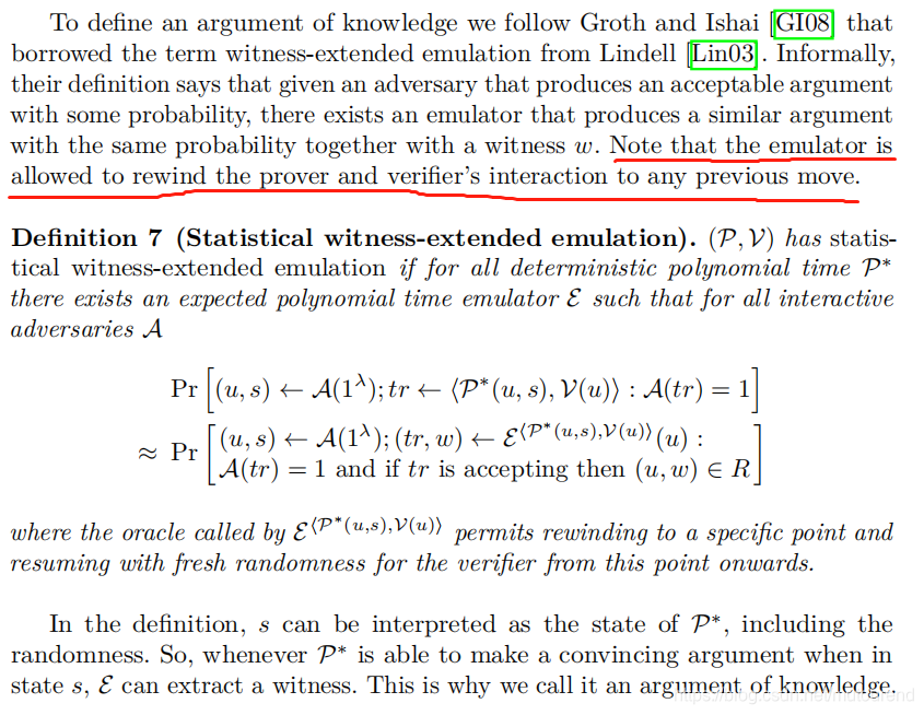
Argument of knowledge定义:
-
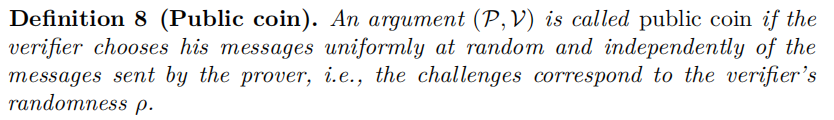
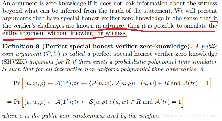
Public coin 和 Perfect special honest verifier zero-knowledge 定义:
-
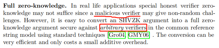
Full zero-knowledge 定义:
-
Fiat-Shamir heuristic 定义:
The Fiat-Shamir transformation takes an interactive public coin argument and replaces the challenges with the output of a cryptographic hash function. The idea is that the hash function will produce random looking output and therefore be a suitable replacement for the verifier.The Fiat-Shamir heuristic yields a non-interactive zero-knowledge argument in the random oracle model [BR93].
本文可借助Fiat-Shamir heuristic,将logarithmic number of move转换为single one move的argument。
1.4 相关假设
-
Discrete Logarithm Assumption:
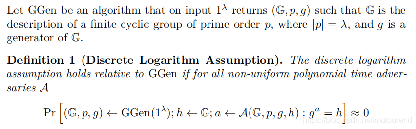
-
Discrete Logarithm Relation Assumption:(与Discrete Logarithm Assumption 等价)

-
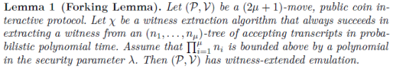
A general forking lemma定义:
假设有 ( 2 μ + 1 ) (2\mu+1) (2μ+1)-move public-coin argument,该argument有 μ \mu μ 个challenges —— 依次为 x 1 , ⋯ , x μ x_1,\cdots,x_{\mu} x1,⋯,xμ。
对于 1 ≤ i ≤ μ 1\leq i\leq \mu 1≤i≤μ,有 n i ≥ 1 n_i\geq 1 ni≥1,将具有 ∏ i = 1 μ n i \prod_{i=1}^{\mu}n_i ∏i=1μni 个accepting transcripts with challenges以tree 方式表示,该tree的depth为 μ \mu μ,具有的leaves数量为 ∏ i = 1 μ n i \prod_{i=1}^{\mu}n_i ∏i=1μni,该tree的根表示为the statement。每个depth i < μ i<\mu i<μ 的node,有 n i n_i ni 个children,每个都labelled with a distinct value for the i i ith challenge x i x_i xi。
可将其理解为 ( n 1 , ⋯ , n μ ) (n_1,\cdots,n_{\mu}) (n1,⋯,nμ)-tree of accepting transcripts。可理解为对Sigma-protocol来说,其 μ = 1 , n = 2 \mu=1,n=2 μ=1,n=2 的generalisation。
本文所构建的arguments均可以 extract the witness from an appropriate tree of accepting transcripts。
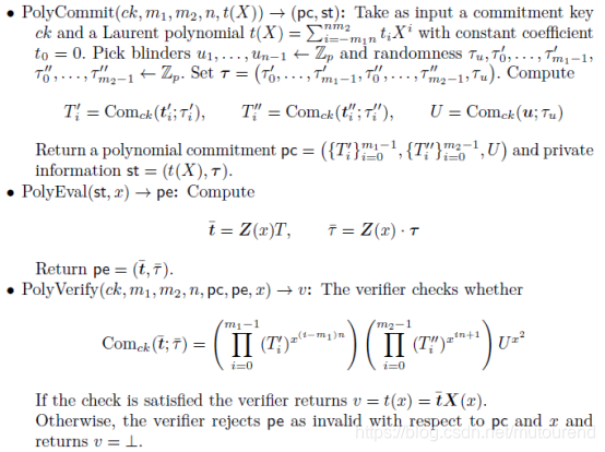
2. Polynomial commitment
Polynomial commitment 基本流程为:
- 1)commit to a polynomial t ( X ) t(X) t(X);
- 2)reveal the evaluation of t ( X ) t(X) t(X) at any point x ∈ Z p ∗ x\in\mathbb{Z}_p* x∈Zp∗;
- 3)同时提供a proof 允许Verifier check that the evaluation is correct with respect to the committed t ( X ) t(X) t(X)。
将 t ( X ) t(X) t(X)理解为是具有negative degree的Laurent polynomials, t ( X ) ∈ Z p [ X , X − 1 ] t(X)\in\mathbb{Z}_p[X,X^{-1}] t(X)∈Zp[X,X−1]。(可参见博客 Laurent polynomial劳伦特多项式)
t ( X ) = ∑ k = − d 1 d 2 t k X k = t − d 1 X − d 1 + t − d 1 + 1 X − d 1 + 1 + ⋯ + t 0 + t 1 X + ⋯ + t d 2 X d 2 t(X)=\sum_{k=-d_1}^{d_2}t_kX^k=t_{-d_1}X^{-d_1}+t_{-d_1+1}X^{-d_1+1}+\cdots+t_0+t_1X+\cdots+t_{d_2}X^{d_2} t(X)=∑k=−d1d2tkXk=t−d1X−d1+t−d1+1X−d1+1+⋯+t0+t1X+⋯+td2Xd2
由于有 C o m ( a 1 m 1 + a 2 m 2 ) = C o m ( m 1 ) a 1 ⋅ C o m ( m 2 ) a 2 Com(a_1m_1+a_2m_2)=Com(m_1)^{a_1}\cdot Com(m_2)^{a_2} Com(a1m1+a2m2)=Com(m1)a1⋅Com(m2)a2
最简单的方法是对 t ( X ) t(X) t(X)的每个系数分别进行commitment,然后可以利用commitment的同态属性直接verify the evaluation of t ( X ) t(X) t(X) at any particular point。存在的问题是需要发送 d d d 个 group elements,其中 d d d 为the number of non-zero coefficients in t ( X ) t(X) t(X)。
本文构建的算法其communication cost 可由 O ( d ) O(d) O(d) 降为 O ( d ) O(\sqrt{d}) O(d),其中 d = d 2 + d 1 d=d_2+d_1 d=d2+d1。
分两个阶段来看:
(1)针对standard polynomial t ( X ) = ∑ k = 0 d t k X k t(X)=\sum_{k=0}^{d}t_kX^k t(X)=∑k=0dtkXk,假设 d + 1 = m n d+1=mn d+1=mn,可将 t ( X ) t(X) t(X)表示为:
t ( X ) = ∑ i = 0 m − 1 ∑ j = 0 n − 1 t i , j X i n + j t(X)=\sum_{i=0}^{m-1}\sum_{j=0}^{n-1}t_{i,j}X^{in+j} t(X)=∑i=0m−1∑j=0n−1ti,jXin+j,将其系数以 m × n m\times n m×n矩阵表示:
T = ( t 0 , 0 t 0 , 1 ⋯ t 0 , n − 1 t 1 , 0 t 1 , 1 ⋯ t 1 , n − 1 ⋮ ⋮ ⋮ t m − 1 , 0 t m − 1 , 1 ⋯ t m − 1 , n − 1 ) \mathbf{T}=\begin{pmatrix} t_{0,0} & t_{0,1} & \cdots & t_{0,n-1}\\ t_{1,0} & t_{1,1} & \cdots & t_{1,n-1}\\ \vdots & \vdots & & \vdots\\ t_{m-1,0} & t_{m-1,1} & \cdots & t_{m-1,n-1} \end{pmatrix} T=⎝⎜⎜⎜⎛t0,0t1,0⋮tm−1,0t0,1t1,1⋮tm−1,1⋯⋯⋯t0,n−1t1,n−1⋮tm−1,n−1⎠⎟⎟⎟⎞
此时, t ( X ) t(X) t(X) 可evaluate by multiplying the matrix by row and column vectors:
t ( X ) = ( 1 X n ⋯ X ( m − 1 ) n ) ( t 0 , 0 t 0 , 1 ⋯ t 0 , n − 1 t 1 , 0 t 1 , 1 ⋯ t 1 , n − 1 ⋮ ⋮ ⋮ t m − 1 , 0 t m − 1 , 1 ⋯ t m − 1 , n − 1 ) ( 1 X ⋮ X n − 1 ) t(X)= \begin{pmatrix} 1 & X^n & \cdots & X^{(m-1)n} \end{pmatrix}\begin{pmatrix} t_{0,0} & t_{0,1} & \cdots & t_{0,n-1}\\ t_{1,0} & t_{1,1} & \cdots & t_{1,n-1}\\ \vdots & \vdots & & \vdots\\ t_{m-1,0} & t_{m-1,1} & \cdots & t_{m-1,n-1} \end{pmatrix}\begin{pmatrix} 1\\ X\\ \vdots\\ X^{n-1} \end{pmatrix} t(X)=(1Xn⋯X(m−1)n)⎝⎜⎜⎜⎛t0,0t1,0⋮tm−1,0t0,1t1,1⋮tm−1,1⋯⋯⋯t0,n−1t1,n−1⋮tm−1,n−1⎠⎟⎟⎟⎞⎝⎜⎜⎜⎛1X⋮Xn−1⎠⎟⎟⎟⎞
基本思路为:
- 对系数矩阵 T \mathbf{T} T的每行进行commitment,相应的commitment值为 T 0 , ⋯ , T m − 1 T_0,\cdots,T_{m-1} T0,⋯,Tm−1;
- 对evaluation point x ∈ Z p x\in\mathbb{Z}_p x∈Zp,利用commitment的同态属性,可知,对应如下vector 的commitment值为 C o m ( t ˉ ⃗ ) = ∏ i = 1 m − 1 T i x i n Com(\vec{\bar{t}})=\prod_{i=1}^{m-1}T_i^{x^{in}} Com(tˉ)=∏i=1m−1Tixin:
t ˉ ⃗ = ( 1 x n ⋯ x ( m − 1 ) n ) ( t 0 , 0 t 0 , 1 ⋯ t 0 , n − 1 t 1 , 0 t 1 , 1 ⋯ t 1 , n − 1 ⋮ ⋮ ⋮ t m − 1 , 0 t m − 1 , 1 ⋯ t m − 1 , n − 1 ) \vec{\bar{t}}=\begin{pmatrix} 1 & x^n & \cdots & x^{(m-1)n} \end{pmatrix}\begin{pmatrix} t_{0,0} & t_{0,1} & \cdots & t_{0,n-1}\\ t_{1,0} & t_{1,1} & \cdots & t_{1,n-1}\\ \vdots & \vdots & & \vdots\\ t_{m-1,0} & t_{m-1,1} & \cdots & t_{m-1,n-1} \end{pmatrix} tˉ=(1xn⋯x(m−1)n)⎝⎜⎜⎜⎛t0,0t1,0⋮tm−1,0t0,1t1,1⋮tm−1,1⋯⋯⋯t0,n−1t1,n−1⋮tm−1,n−1⎠⎟⎟⎟⎞ - Prover可直接open C o m ( t ˉ ⃗ ) Com(\vec{\bar{t}}) Com(tˉ),然后Verifier就很容易计算出evaluation值 v = t ( x ) = t ˉ ⃗ ( 1 x ⋮ x n − 1 ) v=t(x)= \vec{\bar{t}}\begin{pmatrix} 1\\ x\\ \vdots\\ x^{n-1} \end{pmatrix} v=t(x)=tˉ⎝⎜⎜⎜⎛1x⋮xn−1⎠⎟⎟⎟⎞
- 此时,Prover若直接open C o m ( t ˉ ⃗ ) Com(\vec{\bar{t}}) Com(tˉ),将会造成 t ( X ) t(X) t(X)系数的部分泄露。(如设置 x = 0 x=0 x=0,则系数 t 0 , 0 , t 0 , 1 , ⋯ , t 0 , n − 1 t_{0,0},t_{0,1},\cdots,t_{0,n-1} t0,0,t0,1,⋯,t0,n−1将会泄露)
因此,需要在系数矩阵 T \mathbf{T} T中引入blinding values u 1 , ⋯ , u n − 1 u_1,\cdots,u_{n-1} u1,⋯,un−1 来hide the weighted sum of the coefficients in each column。同时,要保证这些blinding values能相互抵消从而仍然保证多项式的evaluation是正确的。
具体实现方式为:
– 构建 ( m + 1 ) × n (m+1)\times n (m+1)×n的系数矩阵:
T = ( t 0 , 0 t 0 , 1 − u 1 ⋯ t 0 , n − 2 − u n − 2 t 0 , n − 1 − u n − 1 t 1 , 0 t 1 , 1 ⋯ t 1 , n − 2 t 1 , n − 1 ⋮ ⋮ ⋮ t m − 1 , 0 t m − 1 , 1 ⋯ t m − 1 , n − 2 t m − 1 , n − 1 u 1 u 2 ⋯ u n − 1 0 ) \mathbf{T}=\begin{pmatrix} t_{0,0} & t_{0,1}-u_1 & \cdots & t_{0,n-2}-u_{n-2} & t_{0,n-1}-u_{n-1}\\ t_{1,0} & t_{1,1} & \cdots & t_{1,n-2} & t_{1,n-1}\\ \vdots & \vdots & & & \vdots\\ t_{m-1,0} & t_{m-1,1} & \cdots & t_{m-1,n-2} & t_{m-1,n-1}\\ u_1 & u_2 & \cdots & u_{n-1} & 0 \end{pmatrix} T=⎝⎜⎜⎜⎜⎜⎛t0,0t1,0⋮tm−1,0u1t0,1−u1t1,1⋮tm−1,1u2⋯⋯⋯⋯t0,n−2−un−2t1,n−2tm−1,n−2un−1t0,n−1−un−1t1,n−1⋮tm−1,n−10⎠⎟⎟⎟⎟⎟⎞
对系数矩阵 T \mathbf{T} T的每行进行commitment,相应的commitment值为 T 0 , ⋯ , T m − 1 , U T_0,\cdots,T_{m-1},U T0,⋯,Tm−1,U
同时, t ( X ) t(X) t(X)可表示为:
t ( X ) = ( 1 X n ⋯ X ( m − 1 ) n X ) T ( 1 X X 2 ⋮ X n − 1 ) t(X)= \begin{pmatrix} 1 & X^n & \cdots & X^{(m-1)n} & X \end{pmatrix}\mathbf{T}\begin{pmatrix} 1\\ X\\ X^2\\ \vdots\\ X^{n-1} \end{pmatrix} t(X)=(1Xn⋯X(m−1)nX)T⎝⎜⎜⎜⎜⎜⎛1XX2⋮Xn−1⎠⎟⎟⎟⎟⎟⎞
– 对evaluation point x ∈ Z p x\in\mathbb{Z}_p x∈Zp,利用commitment的同态属性,可知,对应如下vector 的commitment值为 C o m ( t ˉ ⃗ ) = U x ∏ i = 1 m − 1 T i x i n Com(\vec{\bar{t}})=U^x\prod_{i=1}^{m-1}T_i^{x^{in}} Com(tˉ)=Ux∏i=1m−1Tixin:
t ˉ ⃗ = ( 1 X n ⋯ X ( m − 1 ) n X ) T \vec{\bar{t}}=\begin{pmatrix} 1 & X^n & \cdots & X^{(m-1)n} & X \end{pmatrix}\mathbf{T} tˉ=(1Xn⋯X(m−1)nX)T
– 此时,Prover直接reveal the vector t ˉ ⃗ \vec{\bar{t}} tˉ,就不会造成 t ( X ) t(X) t(X)系数的泄露了。【 x = 0 x=0 x=0时 t 0 , 0 t{0,0} t0,0不算泄露。】
然后Verifier就很容易计算出evaluation值 v = t ( x ) = t ˉ ⃗ ( 1 x ⋮ x n − 1 ) v=t(x)= \vec{\bar{t}}\begin{pmatrix} 1\\ x\\ \vdots\\ x^{n-1} \end{pmatrix} v=t(x)=tˉ⎝⎜⎜⎜⎛1x⋮xn−1⎠⎟⎟⎟⎞。
(2)由standard polynomial 扩展至 Laurent polynomial,其中 t 0 = 0 t_0=0 t0=0。
t ( X ) = ∑ k = − d 1 d 2 t k X k = t − d 1 X − d 1 + t − d 1 + 1 X − d 1 + 1 + ⋯ + t 0 + t 1 X + ⋯ + t d 2 X d 2 t(X)=\sum_{k=-d_1}^{d_2}t_kX^k=t_{-d_1}X^{-d_1}+t_{-d_1+1}X^{-d_1+1}+\cdots+t_0+t_1X+\cdots+t_{d_2}X^{d_2} t(X)=∑k=−d1d2tkXk=t−d1X−d1+t−d1+1X−d1+1+⋯+t0+t1X+⋯+td2Xd2
-
取 m 1 , m 2 , n m_1,m_2,n m1,m2,n均为正整数,且满足 d 1 = n m 1 , d 2 = n m 2 d_1=nm_1,d_2=nm_2 d1=nm1,d2=nm2, t ( X ) t(X) t(X) 可表示为:
t ( X ) = X − m 1 n t ′ ( X ) + X t ′ ′ ( X ) t(X)=X^{-m_1n}t'(X)+Xt''(X) t(X)=X−m1nt′(X)+Xt′′(X),其中 t ′ ( X ) = ∑ i = 0 m 1 − 1 ∑ j = 0 n − 1 t i , j ′ X i n + j , t ′ ′ ( X ) = ∑ i = 0 m 2 − 1 ∑ j = 0 n − 1 t i , j ′ ′ X i n + j t'(X)=\sum_{i=0}^{m_1-1}\sum_{j=0}^{n-1}t'_{i,j}X^{in+j}, t''(X)=\sum_{i=0}^{m_2-1}\sum_{j=0}^{n-1}t''_{i,j}X^{in+j} t′(X)=∑i=0m1−1∑j=0n−1ti,j′Xin+j,t′′(X)=∑i=0m2−1∑j=0n−1ti,j′′Xin+j
可将 t ′ ( X ) t'(X) t′(X)和 t ′ ′ ( X ) t''(X) t′′(X)的系数添加blind values后以 ( m 1 + m 2 ) × n + 1 (m_1+m_2)\times n+1 (m1+m2)×n+1的系数矩阵表示:
T = ( t 0 , 0 ′ t 0 , 1 ′ ⋯ t 0 , n − 1 ′ t 1 , 0 ′ t 1 , 1 ′ ⋯ t 1 , n − 1 ′ ⋮ ⋮ ⋮ t m 1 − 1 , 0 ′ t m 1 − 1 , 1 ′ ⋯ t m 1 − 1 , n − 1 ′ t 0 , 0 ′ ′ t 0 , 1 ′ ′ − u 1 ⋯ t 0 , n − 1 ′ ′ − u n − 1 t 1 , 0 ′ ′ t 1 , 1 ′ ′ ⋯ t 1 , n − 1 ′ ′ ⋮ ⋮ ⋮ t m 2 − 1 , 0 ′ ′ t m 2 − 1 , 1 ′ ′ ⋯ t m 2 − 1 , n − 1 ′ ′ u 1 u 2 ⋯ 0 ) = ( t ⃗ 0 ′ t ⃗ 1 ′ ⋮ t ⃗ m 1 − 1 ′ t ⃗ 0 ′ ′ t ⃗ 1 ′ ′ ⋮ t m 2 − 1 ⃗ ′ ′ u ⃗ ) \mathbf{T}=\begin{pmatrix} t'_{0,0} & t'_{0,1} & \cdots & t'_{0,n-1}\\ t'_{1,0} & t'_{1,1} & \cdots & t'_{1,n-1}\\ \vdots & \vdots & & \vdots\\ t'_{m_1-1,0} & t'_{m_1-1,1} & \cdots & t'_{m_1-1,n-1}\\ t''_{0,0} & t''_{0,1}-u_1 & \cdots & t''_{0,n-1}-u_{n-1}\\ t''_{1,0} & t''_{1,1} & \cdots & t''_{1,n-1}\\ \vdots & \vdots & & \vdots\\ t''_{m_2-1,0} & t''_{m_2-1,1} & \cdots & t''_{m_2-1,n-1}\\ u_1 & u_2 & \cdots & 0 \end{pmatrix}= \begin{pmatrix} \vec{t}_0'\\ \vec{t}_1'\\ \vdots\\ \vec{t}_{m_1-1}'\\ \vec{t}_0''\\ \vec{t}_1''\\ \vdots\\ \vec{t_{m_2-1}}''\\ \vec{u} \end{pmatrix} T=⎝⎜⎜⎜⎜⎜⎜⎜⎜⎜⎜⎜⎜⎜⎜⎛t0,0′t1,0′⋮tm1−1,0′t0,0′′t1,0′′⋮tm2−1,0′′u1t0,1′t1,1′⋮tm1−1,1′t0,1′′−u1t1,1′′⋮tm2−1,1′′u2⋯⋯⋯⋯⋯⋯⋯t0,n−1′t1,n−1′⋮tm1−1,n−1′t0,n−1′′−un−1t1,n−1′′⋮tm2−1,n−1′′0⎠⎟⎟⎟⎟⎟⎟⎟⎟⎟⎟⎟⎟⎟⎟⎞=⎝⎜⎜⎜⎜⎜⎜⎜⎜⎜⎜⎜⎜⎜⎜⎜⎛t0′t1′⋮tm1−1′t0′′t1′′⋮tm2−1′′u⎠⎟⎟⎟⎟⎟⎟⎟⎟⎟⎟⎟⎟⎟⎟⎟⎞
定义 vectors:
Z ⃗ = Z ( X ) ⃗ = ( X − m 1 n , X − ( m 1 − 1 ) n , ⋯ , X − n , X , X n + 1 , ⋯ , X ( m 2 − 1 ) n + 1 , X 2 ) \vec{Z}=\vec{Z(X)}=(X^{-m_1n},X^{-(m_1-1)n},\cdots,X^{-n},X,X^{n+1},\cdots,X^{(m_2-1)n+1},X^2) Z=Z(X)=(X−m1n,X−(m1−1)n,⋯,X−n,X,Xn+1,⋯,X(m2−1)n+1,X2)
X ⃗ = X ( X ) ⃗ = ( 1 X ⋮ X n − 1 ) \vec{X}=\vec{X(X)}=\begin{pmatrix} 1\\ X\\ \vdots\\ X^{n-1} \end{pmatrix} X=X(X)=⎝⎜⎜⎜⎛1X⋮Xn−1⎠⎟⎟⎟⎞
最终, t ( X ) t(X) t(X)可表示为:
t ( X ) = Z ⃗ T X ⃗ t(X)=\vec{Z}\mathbf{T}\vec{X} t(X)=ZTX -
对系数矩阵 T \mathbf{T} T逐行commit,相应的commitment值为 T 0 ′ , ⋯ , T m 1 − 1 ′ , T 0 ′ ′ , ⋯ , T m 2 − 1 ′ ′ , U T_0',\cdots,T_{m_1-1}',T_0'',\cdots,T_{m_2-1}'',U T0′,⋯,Tm1−1′,T0′′,⋯,Tm2−1′′,U。
-
对vector t ˉ ⃗ = Z ⃗ T \vec{\bar{t}}=\vec{Z}\mathbf{T} tˉ=ZT 的 commitment 值为 ( ∏ i = 0 m 1 − 1 ( T i ′ ) x ( i − m 1 ) n ) ( ∏ i = 0 m 2 − 1 ( T i ′ ′ ) x i n + 1 ) U x 2 (\prod_{i=0}^{m_1-1}(T_i')^{x^{(i-m_1)n}})(\prod_{i=0}^{m_2-1}(T_i'')^{x^{in+1}})U^{x^2} (∏i=0m1−1(Ti′)x(i−m1)n)(∏i=0m2−1(Ti′′)xin+1)Ux2。
-
Prover直接reveal the vector t ˉ ⃗ \vec{\bar{t}} tˉ,然后Verifier就很容易计算出evaluation值 v = t ( x ) = t ˉ ⃗ X ( x ) ⃗ = t ˉ ⃗ ( 1 x ⋮ x n − 1 ) v=t(x)= \vec{\bar{t}}\vec{X(x)}= \vec{\bar{t}}\begin{pmatrix} 1\\ x\\ \vdots\\ x^{n-1} \end{pmatrix} v=t(x)=tˉX(x)=tˉ⎝⎜⎜⎜⎛1x⋮xn−1⎠⎟⎟⎟⎞。
由于已在系数矩阵 T \mathbf{T} T中增加了blind values u 1 , ⋯ , u n − 1 u_1,\cdots, u_{n-1} u1,⋯,un−1,实现了hide the weighted sums of each column,从而使得Verifier is able to compute t ( x ) t(x) t(x) without gaining additional information about its coefficients。
整个polynomial commitment的详细流程为:
以上协议具有如下特性:
- Perfect completeness;
- Statistical ( m 1 + m 2 ) n + 1 (m_1+m_2)n+1 (m1+m2)n+1-Special Soundness;
- Perfect Special Honest Verifier Zero Knowledge。
以上协议的开销主要为:
PolyCommit中的 p c ⃗ \vec{pc} pc中包含 m 1 + m 2 + 1 m_1+m_2+1 m1+m2+1 个group elements;PolyEval中的 p e ⃗ \vec{pe} pe中包含 n + 1 n+1 n+1 个field elements;PolyCommit中的 p c ⃗ \vec{pc} pc的计算开销主要在于计算commitments T i ’ T_i’ Ti’和 T i ’ ’ T_i’’ Ti’’,对应为 m 1 + m 2 m_1+m_2 m1+m2 个 n n n-wide multi-exponentiations。采用[Lim00, M¨ol01,MR08]中的multi-exponentiation技术,最终总的开销大概在 ( m 1 + m 2 ) n log n \frac{(m_1+m_2)n}{\log n} logn(m1+m2)n个group expentiations。PolyEval中的 p e ⃗ \vec{pe} pe的计算开销主要在于计算 Z ⃗ T \vec{Z}\mathbf{T} ZT,需要 n ( m 1 + m 2 ) n(m_1+m_2) n(m1+m2) 个field multiplications。PolyVerify中的主要计算开销在于verification equation中的multi-exponentiations,大概需要 m 1 + m 2 + n log ( m 1 + m 2 + n ) \frac{m_1+m_2+n}{\log (m_1+m_2+n)} log(m1+m2+n)m1+m2+n 个group exponentiations。
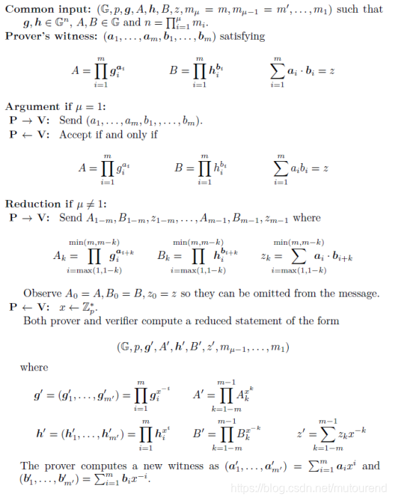
3. Inner product argument
基本信息为:
public info: z ∈ Z p , A , B ∈ G , g ⃗ , h ⃗ ∈ G n z\in\mathbb{Z}_p,A,B\in\mathbb{G},\vec{g},\vec{h}\in\mathbb{G}^n z∈Zp,A,B∈G,g,h∈Gn
private info: a ⃗ , b ⃗ \vec{a},\vec{b} a,b
relation: A = g ⃗ a ⃗ ∧ B = h ⃗ b ⃗ ∧ a ⃗ ⋅ b ⃗ = z A=\vec{g}^{\vec{a}}\wedge B=\vec{h}^{\vec{b}}\wedge \vec{a}\cdot\vec{b}=z A=ga∧B=hb∧a⋅b=z
当不要求zero-knowledge时,Prover可直接将 a ⃗ , b ⃗ \vec{a},\vec{b} a,b发送给Verifier,相应的communication cost为 O ( 2 n ) O(2n) O(2n)。本文可通过增加interaction来减少communication cost 至 O ( n ) O(\sqrt{n}) O(n),其中 n n n为vector length。
本文构建的inner product argument,是基于Bayer和Groth 2012年论文《Efficient zero-knowledge argument for correctness of a shuffle》(参见博客 Efficient Zero-Knowledge Argument for Correctness of a Shuffle学习笔记(1))中类似的2-move reduction to smaller statement技术。即:
It will suffice for the prover to reveal the witness for the smaller statement in order to convince the verifier about the validity of the original statement。
在整个argument中,Prover和Verifier都递归地 run the reduction to obtain increasingly smaller statements,然后最后Prover reveal a witness for a very small statement。最终需要 O ( log n ) O(\log n) O(logn)个move,总的communication cost为 O ( log n ) O(\log n) O(logn) 个 group和field elements。
基本思路为:
Prover和Verifier的common input 为 ( G , p , g ⃗ , A , h ⃗ , B , z , m ) (\mathbb{G},p,\vec{g},A,\vec{h},B,z,m) (G,p,g,A,h,B,z,m),其中 m m m可整除 n n n。对应的 g ⃗ = ( g ⃗ 1 , ⋯ , g ⃗ m ) , h ⃗ = ( h ⃗ 1 , ⋯ , h ⃗ m ) , a ⃗ = ( a ⃗ 1 , ⋯ , a ⃗ m ) , b ⃗ = ( b ⃗ 1 , ⋯ , b ⃗ m ) \vec{g}=(\vec{g}_1,\cdots,\vec{g}_m),\vec{h}=(\vec{h}_1,\cdots,\vec{h}_m),\vec{a}=(\vec{a}_1,\cdots,\vec{a}_m),\vec{b}=(\vec{b}_1,\cdots,\vec{b}_m) g=(g1,⋯,gm),h=(h1,⋯,hm),a=(a1,⋯,am),b=(b1,⋯,bm),其中每个 g ⃗ i , h ⃗ i \vec{g}_i,\vec{h}_i gi,hi的size为 n m \frac{n}{m} mn。
转为证明:
Public info: z ∈ Z p , A , B ∈ G , g ⃗ , h ⃗ ∈ G n z\in\mathbb{Z}_p,A,B\in\mathbb{G},\vec{g},\vec{h}\in\mathbb{G}^n z∈Zp,A,B∈G,g,h∈Gn
Private info: a ⃗ = ( a ⃗ 1 , ⋯ , a ⃗ m ) , b ⃗ = ( b ⃗ 1 , ⋯ , b ⃗ m ) \vec{a}=(\vec{a}_1,\cdots,\vec{a}_m),\vec{b}=(\vec{b}_1,\cdots,\vec{b}_m) a=(a1,⋯,am),b=(b1,⋯,bm)
Relation: A = g ⃗ a ⃗ = ∏ i = 1 m g ⃗ i a ⃗ i ∧ B = h ⃗ b ⃗ = ∏ i = 1 m h ⃗ i b ⃗ i ∧ a ⃗ ⋅ b ⃗ = ∑ i = 1 m a ⃗ i ⋅ b ⃗ i = z A=\vec{g}^{\vec{a}}=\prod_{i=1}^{m}\vec{g}_i^{\vec{a}_i}\wedge B=\vec{h}^{\vec{b}}=\prod_{i=1}^{m}\vec{h}_i^{\vec{b}_i}\wedge \vec{a}\cdot\vec{b}=\sum_{i=1}^{m}\vec{a}_i\cdot\vec{b}_i=z A=ga=∏i=1mgiai∧B=hb=∏i=1mhibi∧a⋅b=∑i=1mai⋅bi=z
将其展开为矩阵,主对角线上的元素即为相应的vector commitment。
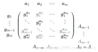
- Prover:for k = 1 − m , ⋯ , m − 1 k=1-m,\cdots,m-1 k=1−m,⋯,m−1,计算 A k = ∏ i = m a x ( 1 , 1 − k ) m i n ( m , m − k ) g ⃗ i a ⃗ i + k , B k = ∏ i = m a x ( 1 , 1 − k ) m i n ( m , m − k ) h ⃗ i b ⃗ i + k A_k=\prod_{i=max(1,1-k)}^{min(m,m-k)}\vec{g}_i^{\vec{a}_{i+k}}, B_k=\prod_{i=max(1,1-k)}^{min(m,m-k)}\vec{h}_i^{\vec{b}_{i+k}} Ak=∏i=max(1,1−k)min(m,m−k)giai+k,Bk=∏i=max(1,1−k)min(m,m−k)hibi+k。将所有的 A k A_k Ak 发送给Verifier。其中 A 0 = A , B 0 = B A_0=A,B_0=B A0=A,B0=B为public info。
- Verifier:发送 challenge x ← Z p ∗ x\leftarrow \mathbb{Z}_p* x←Zp∗。
- Prover和Verifier:同时计算 g ⃗ ′ = ∏ i = 1 m g ⃗ i x − i , A ′ = ∏ k = 1 − m m − 1 A k x k , h ⃗ ′ = ∏ i = 1 m h ⃗ i x i , B ′ = ∏ k = 1 − m m − 1 B k x − k \vec{g}'=\prod_{i=1}^{m}\vec{g}_i^{x^{-i}},A'=\prod_{k=1-m}^{m-1}A_k^{x^k},\vec{h}'=\prod_{i=1}^{m}\vec{h}_i^{x^{i}},B'=\prod_{k=1-m}^{m-1}B_k^{x^{-k}} g′=∏i=1mgix−i,A′=∏k=1−mm−1Akxk,h′=∏i=1mhixi,B′=∏k=1−mm−1Bkx−k。
- Prover:构建新的witness a ⃗ ′ = ∑ i = 1 m a ⃗ i x i , b ⃗ ′ = ∑ i = 1 m b ⃗ i x − i \vec{a}'=\sum_{i=1}^{m}\vec{a}_ix^i, \vec{b}'=\sum_{i=1}^{m}\vec{b}_ix^{-i} a′=∑i=1maixi,b′=∑i=1mbix−i,使得 A ′ = ( g ⃗ ′ ) a ⃗ ′ , B ′ = ( h ⃗ ′ ) b ⃗ ′ A'=(\vec{g}')^{\vec{a}'}, B'=(\vec{h}')^{\vec{b}'} A′=(g′)a′,B′=(h′)b′成立。
- Prover:为了证明 a ⃗ ⋅ b ⃗ = z \vec{a}\cdot\vec{b}=z a⋅b=z,即需要证明 z z z为 a ⃗ ′ ⋅ b ⃗ ′ = ∑ i = 1 m a ⃗ i x i ⋅ ∑ j = 1 m b ⃗ j x − j \vec{a}'\cdot\vec{b}'=\sum_{i=1}^{m}\vec{a}_ix^i\cdot\sum_{j=1}^{m}\vec{b}_jx^{-j} a′⋅b′=∑i=1maixi⋅∑j=1mbjx−j的常量项。
for k = 1 − m , ⋯ , m − 1 k=1-m,\cdots,m-1 k=1−m,⋯,m−1,Prover计算 z k = ∑ i = m a x ( 1 , 1 − k ) m i n ( m , m − k ) a ⃗ i ⋅ b ⃗ i + k z_k=\sum_{i=max(1,1-k)}^{min(m,m-k)}\vec{a}_i\cdot\vec{b}_{i+k} zk=∑i=max(1,1−k)min(m,m−k)ai⋅bi+k。将所有 z k z_k zk发送给Verifier。其中 z 0 = z = ∑ i = 1 m a ⃗ i ⋅ b ⃗ i z_0=z=\sum_{i=1}^{m}\vec{a}_i\cdot\vec{b}_i z0=z=∑i=1mai⋅bi。 - Verifier:计算 z ′ = a ⃗ ′ ⋅ b ⃗ ′ = ∑ k = 1 − m m − 1 z k x − k z'=\vec{a}'\cdot\vec{b}'=\sum_{k=1-m}^{m-1}z_kx^{-k} z′=a′⋅b′=∑k=1−mm−1zkx−k
至此,Prover和Verifier都知道 g ⃗ ′ , A ′ , h ⃗ ′ , B ′ , z ′ \vec{g}',A',\vec{h}',B',z' g′,A′,h′,B′,z′满足 A ′ = g ⃗ ′ a ⃗ ′ ∧ B ′ = h ⃗ ′ b ⃗ ′ ∧ z ′ = a ⃗ ′ ⋅ b ⃗ ′ A'=\vec{g}'^{\vec{a}'}\wedge B'=\vec{h}'^{\vec{b}'}\wedge z'=\vec{a}'\cdot\vec{b}' A′=g′a′∧B′=h′b′∧z′=a′⋅b′,且witness a ⃗ ′ , b ⃗ ′ \vec{a}',\vec{b}' a′,b′的length均为 n m \frac{n}{m} mn。
假设 n = m μ m μ − q ⋯ m 1 n=m_{\mu}m_{\mu-q}\cdots m_1 n=mμmμ−q⋯m1,则可 recursively apply this reduction over the factors of n n n to obtain, after μ − 1 \mu-1 μ−1 iterations,vectors of length m 1 m_1 m1。然后Prover可直接reveal shorter m 1 m_1 m1 length vectors,而不再是 n n n length vectors。
详细的算法实现为:
以上inner product argument协议具有如下属性:
- perfect completeness;
- statistical witness extended emulation。
- 注意:以上argument未实现zero-knowledge。【如博客 Hyrax: Doubly-efficient zkSNARKs without trusted setup学习笔记 4.2节中引入了随机数 r ξ , r τ r_{\xi},r_{\tau} rξ,rτ 来实现honest verifier perfect zero-knowledge。】
以上inner product argument的开销为:
- 整个递归argument需要 2 μ − 1 2\mu-1 2μ−1 moves。
- 所有步骤的communication cost为 4 ∑ i = 2 μ ( m i − 1 ) 4\sum_{i=2}^{\mu}(m_i-1) 4∑i=2μ(mi−1)个group elements和 2 ∑ i = 2 μ ( m i − 1 ) + 2 m 1 2\sum_{i=2}^{\mu}(m_i-1)+2m_1 2∑i=2μ(mi−1)+2m1个field elements。
- 在每个迭代中,Prover的主要computation cost在于计算 A k , B k A_k,B_k Ak,Bk(借助multi-exponentiation技术,需少于 4 ( m μ 2 m μ − 1 ⋯ m 1 ) log ( m μ ⋯ m 1 ) \frac{4(m_{\mu}^2m_{\mu-1}\cdots m_1)}{\log (m_{\mu}\cdots m_1)} log(mμ⋯m1)4(mμ2mμ−1⋯m1)次group exponentiations运算)和计算 z k z_k zk,需要 m μ 2 m μ − 1 ⋯ m 1 m_{\mu}^2m_{\mu-1}\cdots m_1 mμ2mμ−1⋯m1次field multiplication 运算。
- Prover和Verifier在每次迭代中均需要计算 g ⃗ ′ , h ⃗ ′ , A ′ , B ′ , z ′ \vec{g}',\vec{h}',A',B',z' g′,h′,A′,B′,z′,相应的computation cost 主要为 2 ( m μ m μ − 1 ⋯ m 1 ) log m μ \frac{2(m_{\mu}m_{\mu-1}\cdots m_1)}{\log m_{\mu}} logmμ2(mμmμ−1⋯m1)个group exponentiations。
当 m μ = ⋯ = m 1 = m m_{\mu}=\cdots=m_1=m mμ=⋯=m1=m时,Verifier的computation complexity上限为 2 m μ log m m m − 1 \frac{2m^{\mu}}{\log m}\frac{m}{m-1} logm2mμm−1m个group exponentiations,Prover的computation complexity上限为 6 m μ + 1 log m m m − 1 \frac{6m^{\mu+1}}{\log m}\frac{m}{m-1} logm6mμ+1m−1m个group exponentiations和 m μ + 1 m m − 1 m^{\mu+1}\frac{m}{m-1} mμ+1m−1m个field multiplications。
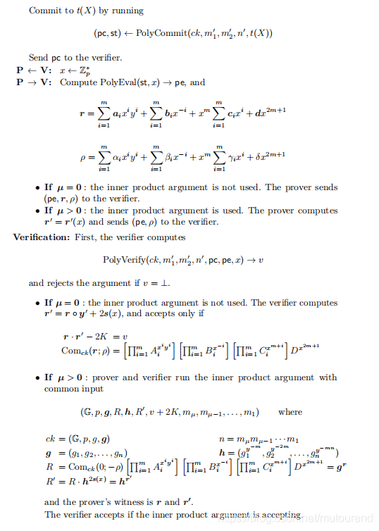
4. 为Arithmetic Circuit Satisfiability构建Logarithmic Communication Argument
Groth 2009年论文《Linear Algebra with Sub-linear Zero-Knowledge Arguments》中基于discrete logarithm assumption的constant round arithmetic circuit 零知识证明算法的communication complexity 为 O ( n ) O(\sqrt{n}) O(n)。(详细可参见博客 Linear Algebra with Sub-linear Zero-Knowledge Arguments学习笔记)
借助第3节的recursive inner product argument,可将communication complexity降为 O ( log n ) O(\log n) O(logn)。
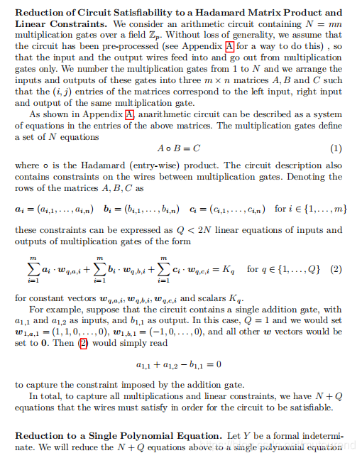
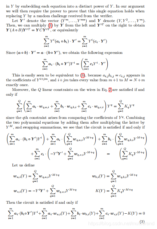
将arithmetic circuit转换为2种类型的equations:
- 乘法门直接表示为 a ⋅ b = c a\cdot b=c a⋅b=c,其中 a , b , c a,b,c a,b,c分别代表the left, right and output wires。可将一系列这样的值以矩阵表示形成a Hadamard matrix product A ∘ B = C \mathbf{A}\circ\mathbf{B}=\mathbf{C} A∘B=C。
- 这种表示方式会存在一些冗余值,如 a wire is the output of one multiplication gate and the input of another 或者 a wire is used as input multiple times。可以通过一系列的linear constraints来跟踪这些冗余:如 the output of the first multiplication gate is the right input of the second,可表示为 c 1 − b 2 = 0 c_1-b_2=0 c1−b2=0。
同时将加法门和常量乘法门以linear constraints表示,最终只需关注非常量乘法门。
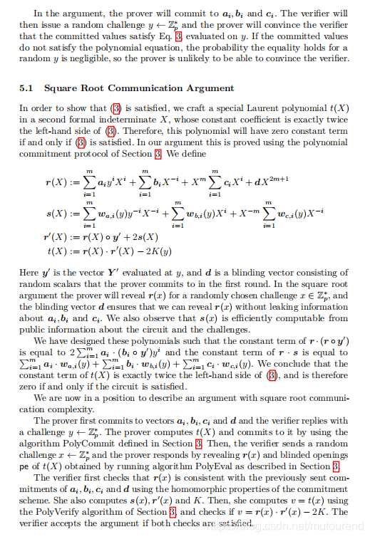
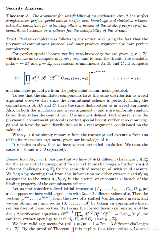
最后,将Hadamard matrix product和linear constraints压缩为a single polynomial equation,以Laurent polynomial 表示(其constant term为 0 0 0)。可采用第2节的polynomial commitment来证明,同时可结合第3节的inner product argument来减少communication cost。
相比于Groth 2009年论文《Linear Algebra with Sub-linear Zero-Knowledge Arguments》的arithmetic circuit算法,主要从以下三方面做了改进:
- 不再需要加法门的input 和 output commitments了。将加法门以linear consistency equation形式来出来,可大幅提高性能。与此同时的研究成果,在Gennaro等人2013年论文《Quadratic span programs and succinct NIZKs without PCPs》中,也是去除了加法门,只不过采用的方式是从circuit中构建 Quadratic Arithmetic Programs。
- 避免对generic linear algebra statements采用黑盒reduction,而是为arithmetic circuit satisfiability直接设计an argument。
本文的square-root argument仅需要5 moves,而Groth 2009年论文《Linear Algebra with Sub-linear Zero-Knowledge Arguments》中的argument需要7 moves。而Seo 2011年论文《Round-efficient sub-linear zero-knowledge arguments for linear algebra》中虽然为5 moves,但是增加了computational cost。 - 可采用第2节的方式来减少polynomial commitment的communication cost。
最终,本文实现的communication complexity为 O ( N ) O(\sqrt{N}) O(N),其中 N N N表示multiplication gate的数量。
假设circuit有 N = m n N=mn N=mn个multiplication gates,Prover在第一轮为make 3 m 3m 3m commitments to wire values,然后提供an opening consisting of n n n field elements to a homomorphic combination of these commitments。当 m ≈ n ≈ N m\approx n\approx \sqrt{N} m≈n≈N时,即具有 O ( N ) O(\sqrt{N}) O(N) communication complexity。
Verifier利用这 n n n个field elements来验证 an inner product relation,为了进一步降低communication cost,可采用第3节中的inner product argument来减少sending field elements的数量。
智能推荐
while循环&CPU占用率高问题深入分析与解决方案_main函数使用while(1)循环cpu占用99-程序员宅基地
文章浏览阅读3.8k次,点赞9次,收藏28次。直接上一个工作中碰到的问题,另外一个系统开启多线程调用我这边的接口,然后我这边会开启多线程批量查询第三方接口并且返回给调用方。使用的是两三年前别人遗留下来的方法,放到线上后发现确实是可以正常取到结果,但是一旦调用,CPU占用就直接100%(部署环境是win server服务器)。因此查看了下相关的老代码并使用JProfiler查看发现是在某个while循环的时候有问题。具体项目代码就不贴了,类似于下面这段代码。while(flag) {//your code;}这里的flag._main函数使用while(1)循环cpu占用99
【无标题】jetbrains idea shift f6不生效_idea shift +f6快捷键不生效-程序员宅基地
文章浏览阅读347次。idea shift f6 快捷键无效_idea shift +f6快捷键不生效
node.js学习笔记之Node中的核心模块_node模块中有很多核心模块,以下不属于核心模块,使用时需下载的是-程序员宅基地
文章浏览阅读135次。Ecmacript 中没有DOM 和 BOM核心模块Node为JavaScript提供了很多服务器级别,这些API绝大多数都被包装到了一个具名和核心模块中了,例如文件操作的 fs 核心模块 ,http服务构建的http 模块 path 路径操作模块 os 操作系统信息模块// 用来获取机器信息的var os = require('os')// 用来操作路径的var path = require('path')// 获取当前机器的 CPU 信息console.log(os.cpus._node模块中有很多核心模块,以下不属于核心模块,使用时需下载的是
数学建模【SPSS 下载-安装、方差分析与回归分析的SPSS实现(软件概述、方差分析、回归分析)】_化工数学模型数据回归软件-程序员宅基地
文章浏览阅读10w+次,点赞435次,收藏3.4k次。SPSS 22 下载安装过程7.6 方差分析与回归分析的SPSS实现7.6.1 SPSS软件概述1 SPSS版本与安装2 SPSS界面3 SPSS特点4 SPSS数据7.6.2 SPSS与方差分析1 单因素方差分析2 双因素方差分析7.6.3 SPSS与回归分析SPSS回归分析过程牙膏价格问题的回归分析_化工数学模型数据回归软件
利用hutool实现邮件发送功能_hutool发送邮件-程序员宅基地
文章浏览阅读7.5k次。如何利用hutool工具包实现邮件发送功能呢?1、首先引入hutool依赖<dependency> <groupId>cn.hutool</groupId> <artifactId>hutool-all</artifactId> <version>5.7.19</version></dependency>2、编写邮件发送工具类package com.pc.c..._hutool发送邮件
docker安装elasticsearch,elasticsearch-head,kibana,ik分词器_docker安装kibana连接elasticsearch并且elasticsearch有密码-程序员宅基地
文章浏览阅读867次,点赞2次,收藏2次。docker安装elasticsearch,elasticsearch-head,kibana,ik分词器安装方式基本有两种,一种是pull的方式,一种是Dockerfile的方式,由于pull的方式pull下来后还需配置许多东西且不便于复用,个人比较喜欢使用Dockerfile的方式所有docker支持的镜像基本都在https://hub.docker.com/docker的官网上能找到合..._docker安装kibana连接elasticsearch并且elasticsearch有密码
随便推点
Python 攻克移动开发失败!_beeware-程序员宅基地
文章浏览阅读1.3w次,点赞57次,收藏92次。整理 | 郑丽媛出品 | CSDN(ID:CSDNnews)近年来,随着机器学习的兴起,有一门编程语言逐渐变得火热——Python。得益于其针对机器学习提供了大量开源框架和第三方模块,内置..._beeware
Swift4.0_Timer 的基本使用_swift timer 暂停-程序员宅基地
文章浏览阅读7.9k次。//// ViewController.swift// Day_10_Timer//// Created by dongqiangfei on 2018/10/15.// Copyright 2018年 飞飞. All rights reserved.//import UIKitclass ViewController: UIViewController { ..._swift timer 暂停
元素三大等待-程序员宅基地
文章浏览阅读986次,点赞2次,收藏2次。1.硬性等待让当前线程暂停执行,应用场景:代码执行速度太快了,但是UI元素没有立马加载出来,造成两者不同步,这时候就可以让代码等待一下,再去执行找元素的动作线程休眠,强制等待 Thread.sleep(long mills)package com.example.demo;import org.junit.jupiter.api.Test;import org.openqa.selenium.By;import org.openqa.selenium.firefox.Firefox.._元素三大等待
Java软件工程师职位分析_java岗位分析-程序员宅基地
文章浏览阅读3k次,点赞4次,收藏14次。Java软件工程师职位分析_java岗位分析
Java:Unreachable code的解决方法_java unreachable code-程序员宅基地
文章浏览阅读2k次。Java:Unreachable code的解决方法_java unreachable code
标签data-*自定义属性值和根据data属性值查找对应标签_如何根据data-*属性获取对应的标签对象-程序员宅基地
文章浏览阅读1w次。1、html中设置标签data-*的值 标题 11111 222222、点击获取当前标签的data-url的值$('dd').on('click', function() { var urlVal = $(this).data('ur_如何根据data-*属性获取对应的标签对象