【吴恩达深度学习】Deep Neural Network for Image Classification: Application-程序员宅基地
技术标签: 人工智能,机器学习,深度学习 算法 深度学习 人工智能
Deep Neural Network for Image Classification: Application
When you finish this, you will have finished the last programming assignment of Week 4, and also the last programming assignment of this course!
You will use the functions you’d implemented in the previous assignment to build a deep network, and apply it to cat vs non-cat classification. Hopefully, you will see an improvement in accuracy relative to your previous logistic regression implementation.
After this assignment you will be able to:
- Build and apply a deep neural network to supervised learning.
Let’s get started!
1 - Packages
Let’s first import all the packages that you will need during this assignment.
- numpy is the fundamental package for scientific computing with Python.
- matplotlib is a library to plot graphs in Python.
- h5py is a common package to interact with a dataset that is stored on an H5 file.
- PIL and scipy are used here to test your model with your own picture at the end.
- dnn_app_utils provides the functions implemented in the “Building your Deep Neural Network: Step by Step” assignment to this notebook.
- np.random.seed(1) is used to keep all the random function calls consistent. It will help us grade your work.
import time
import numpy as np
import h5py
import matplotlib.pyplot as plt
import scipy
from PIL import Image
from scipy import ndimage
from dnn_app_utils_v2 import *

%matplotlib inline
plt.rcParams['figure.figsize'] = (5.0, 4.0) # set default size of plots
plt.rcParams['image.interpolation'] = 'nearest'
plt.rcParams['image.cmap'] = 'gray'

%load_ext autoreload
%autoreload 2

np.random.seed(1)
2 - Dataset
You will use the same “Cat vs non-Cat” dataset as in “Logistic Regression as a Neural Network” (Assignment 2). The model you had built had 70% test accuracy on classifying cats vs non-cats images. Hopefully, your new model will perform a better!
Problem Statement: You are given a dataset (“data.h5”) containing:
- a training set of m_train images labelled as cat (1) or non-cat (0)
- a test set of m_test images labelled as cat and non-cat
- each image is of shape (num_px, num_px, 3) where 3 is for the 3 channels (RGB).
Let’s get more familiar with the dataset. Load the data by running the cell below.
train_x_orig, train_y, test_x_orig, test_y, classes = load_data()
The following code will show you an image in the dataset. Feel free to change the index and re-run the cell multiple times to see other images.
# Example of a picture
index = 7
plt.imshow(train_x_orig[index])
print ("y = " + str(train_y[0,index]) + ". It's a " + classes[train_y[0,index]].decode("utf-8") +  " picture.")
# Explore your dataset
m_train = train_x_orig.shape[0]
num_px = train_x_orig.shape[1]
m_test = test_x_orig.shape[0]

print ("Number of training examples: " + str(m_train))
print ("Number of testing examples: " + str(m_test))
print ("Each image is of size: (" + str(num_px) + ", " + str(num_px) + ", 3)")
print ("train_x_orig shape: " + str(train_x_orig.shape))
print ("train_y shape: " + str(train_y.shape))
print ("test_x_orig shape: " + str(test_x_orig.shape))
print ("test_y shape: " + str(test_y.shape))
As usual, you reshape and standardize the images before feeding them to the network. The code is given in the cell below.
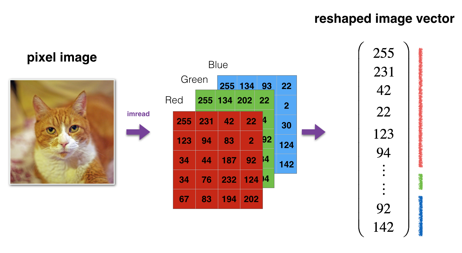
# Reshape the training and test examples
train_x_flatten = train_x_orig.reshape(train_x_orig.shape[0], -1).T   # The "-1" makes reshape flatten the remaining dimensions
test_x_flatten = test_x_orig.reshape(test_x_orig.shape[0], -1).T

# Standardize data to have feature values between 0 and 1.
train_x = train_x_flatten/255.
test_x = test_x_flatten/255.

print ("train_x's shape: " + str(train_x.shape))
print ("test_x's shape: " + str(test_x.shape))
12 , 288 12,288 12,288 equals 64 × 64 × 3 64 \times 64 \times 3 64×64×3 which is the size of one reshaped image vector.
3 - Architecture of your model
Now that you are familiar with the dataset, it is time to build a deep neural network to distinguish cat images from non-cat images.
You will build two different models:
- A 2-layer neural network
- An L-layer deep neural network
You will then compare the performance of these models, and also try out different values for L L L.
Let’s look at the two architectures.
3.1 - 2-layer neural network
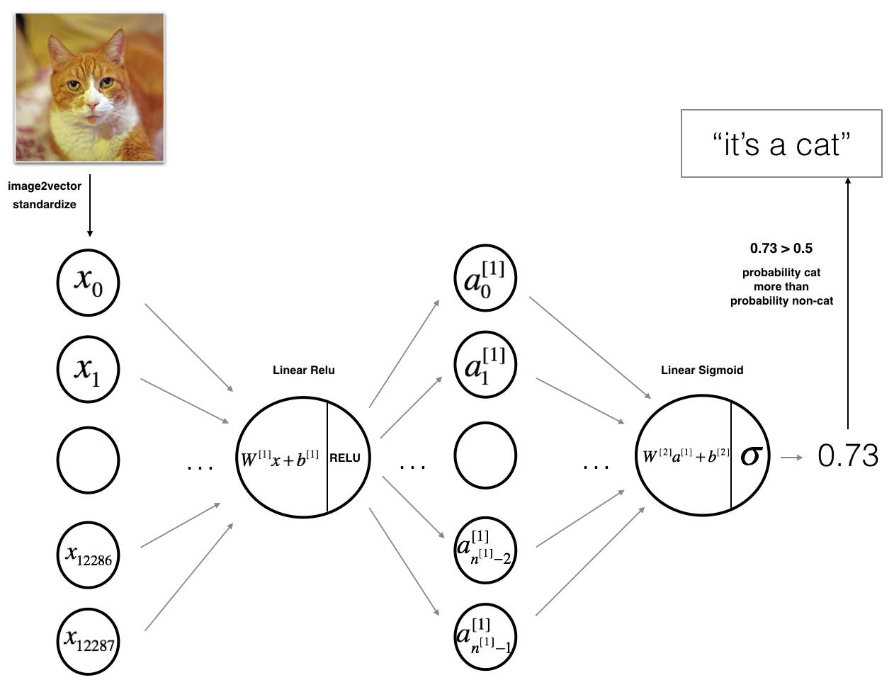
The model can be summarized as: ***INPUT -> LINEAR -> RELU -> LINEAR -> SIGMOID -> OUTPUT***.
Detailed Architecture of figure 2:
- The input is a (64,64,3) image which is flattened to a vector of size ( 12288 , 1 ) (12288,1) (12288,1).
- The corresponding vector: [ x 0 , x 1 , . . . , x 12287 ] T [x_0,x_1,...,x_{12287}]^T [x0,x1,...,x12287]T is then multiplied by the weight matrix W [ 1 ] W^{[1]} W[1] of size ( n [ 1 ] , 12288 ) (n^{[1]}, 12288) (n[1],12288).
- You then add a bias term and take its relu to get the following vector: [ a 0 [ 1 ] , a 1 [ 1 ] , . . . , a n [ 1 ] − 1 [ 1 ] ] T [a_0^{[1]}, a_1^{[1]},..., a_{n^{[1]}-1}^{[1]}]^T [a0[1],a1[1],...,an[1]−1[1]]T.
- You then repeat the same process.
- You multiply the resulting vector by W [ 2 ] W^{[2]} W[2] and add your intercept (bias).
- Finally, you take the sigmoid of the result. If it is greater than 0.5, you classify it to be a cat.
3.2 - L-layer deep neural network
It is hard to represent an L-layer deep neural network with the above representation. However, here is a simplified network representation:
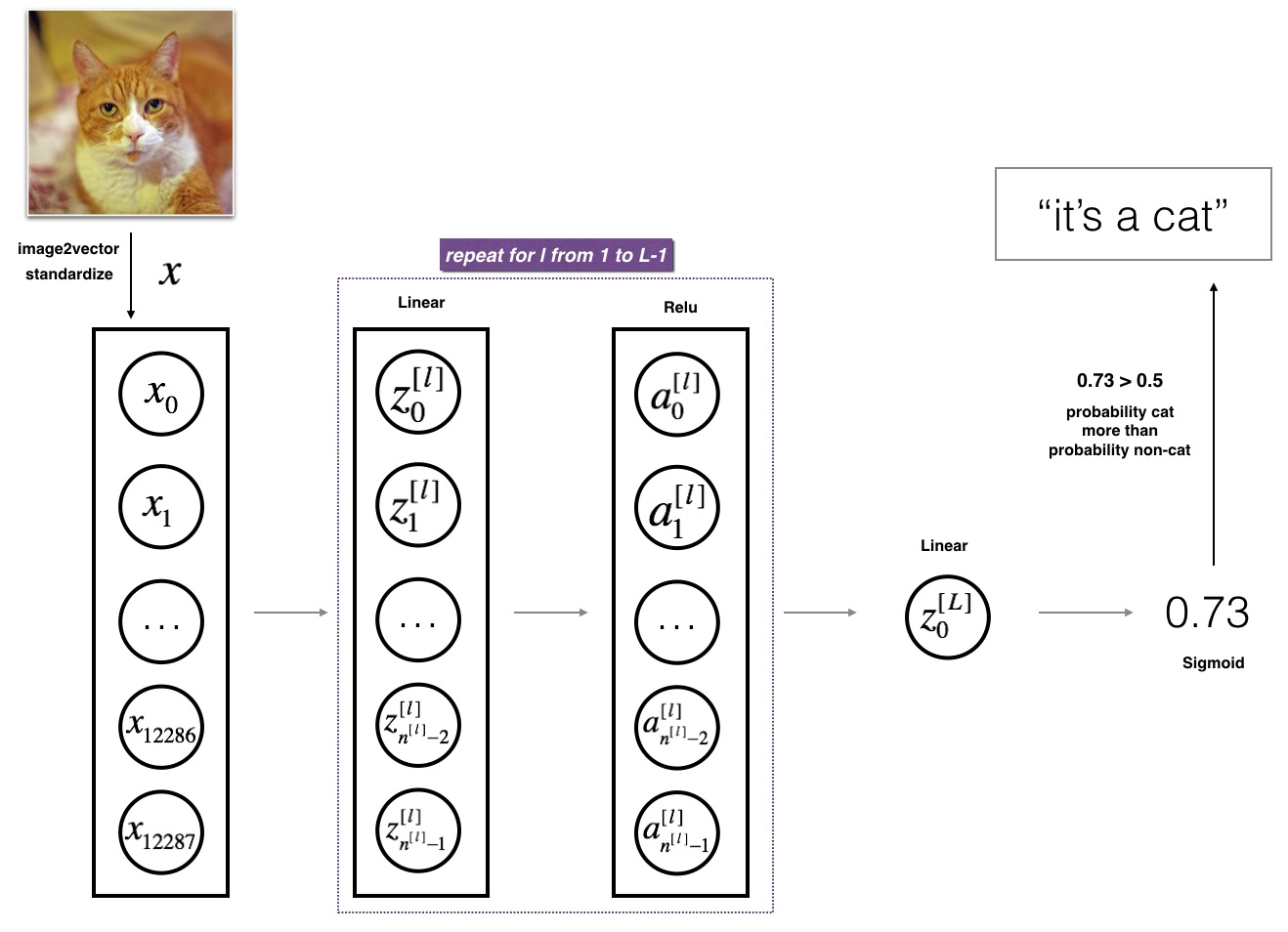
The model can be summarized as: ***[LINEAR -> RELU] $\times$ (L-1) -> LINEAR -> SIGMOID***
Detailed Architecture of figure 3:
- The input is a (64,64,3) image which is flattened to a vector of size (12288,1).
- The corresponding vector: [ x 0 , x 1 , . . . , x 12287 ] T [x_0,x_1,...,x_{12287}]^T [x0,x1,...,x12287]T is then multiplied by the weight matrix W [ 1 ] W^{[1]} W[1] and then you add the intercept b [ 1 ] b^{[1]} b[1]. The result is called the linear unit.
- Next, you take the relu of the linear unit. This process could be repeated several times for each ( W [ l ] , b [ l ] ) (W^{[l]}, b^{[l]}) (W[l],b[l]) depending on the model architecture.
- Finally, you take the sigmoid of the final linear unit. If it is greater than 0.5, you classify it to be a cat.
3.3 - General methodology
As usual you will follow the Deep Learning methodology to build the model:
1. Initialize parameters / Define hyperparameters
2. Loop for num_iterations:
a. Forward propagation
b. Compute cost function
c. Backward propagation
d. Update parameters (using parameters, and grads from backprop)
4. Use trained parameters to predict labels
Let’s now implement those two models!
4 - Two-layer neural network
Question: Use the helper functions you have implemented in the previous assignment to build a 2-layer neural network with the following structure: LINEAR -> RELU -> LINEAR -> SIGMOID. The functions you may need and their inputs are:
def initialize_parameters(n_x, n_h, n_y):
    ...
    return parameters
def linear_activation_forward(A_prev, W, b, activation):
    ...
    return A, cache
def compute_cost(AL, Y):
    ...
    return cost
def linear_activation_backward(dA, cache, activation):
    ...
    return dA_prev, dW, db
def update_parameters(parameters, grads, learning_rate):
    ...
    return parameters
### CONSTANTS DEFINING THE MODEL ####
n_x = 12288     # num_px * num_px * 3
n_h = 7
n_y = 1
layers_dims = (n_x, n_h, n_y)
# GRADED FUNCTION: two_layer_model

def two_layer_model(X, Y, layers_dims, learning_rate = 0.0075, num_iterations = 3000, print_cost=False):
    """
    Implements a two-layer neural network: LINEAR->RELU->LINEAR->SIGMOID.

    Arguments:
    X -- input data, of shape (n_x, number of examples)
    Y -- true "label" vector (containing 0 if cat, 1 if non-cat), of shape (1, number of examples)
    layers_dims -- dimensions of the layers (n_x, n_h, n_y)
    num_iterations -- number of iterations of the optimization loop
    learning_rate -- learning rate of the gradient descent update rule
    print_cost -- If set to True, this will print the cost every 100 iterations

    Returns:
    parameters -- a dictionary containing W1, W2, b1, and b2
    """

    np.random.seed(1)
    grads = {
    }
    costs = []                              # to keep track of the cost
    m = X.shape[1]                           # number of examples
    (n_x, n_h, n_y) = layers_dims

    # Initialize parameters dictionary, by calling one of the functions you'd previously implemented
    ### START CODE HERE ### (≈ 1 line of code)
    parameters=initialize_parameters(n_x,n_h,n_y)
    ### END CODE HERE ###

    # Get W1, b1, W2 and b2 from the dictionary parameters.
    W1 = parameters["W1"]
    b1 = parameters["b1"]
    W2 = parameters["W2"]
    b2 = parameters["b2"]

    # Loop (gradient descent)

    for i in range(0, num_iterations):

        # Forward propagation: LINEAR -> RELU -> LINEAR -> SIGMOID. Inputs: "X, W1, b1". Output: "A1, cache1, A2, cache2".
        ### START CODE HERE ### (≈ 2 lines of code)
        A1,cache1=linear_activation_forward(X,W1,b1,activation="relu")
        A2,cache2=linear_activation_forward(A1,W2,b2,activation="sigmoid")
        ### END CODE HERE ###

        # Compute cost
        ### START CODE HERE ### (≈ 1 line of code)
        cost=compute_cost(A2,Y)
        ### END CODE HERE ###

        # Initializing backward propagation
        dA2 = - (np.divide(Y, A2) - np.divide(1 - Y, 1 - A2))

        # Backward propagation. Inputs: "dA2, cache2, cache1". Outputs: "dA1, dW2, db2; also dA0 (not used), dW1, db1".
        ### START CODE HERE ### (≈ 2 lines of code)
        dA1,dW2,db2=linear_activation_backward(dA2,cache2,activation="sigmoid")
        dA0,dW1,db1=linear_activation_backward(dA1,cache1,activation="relu")
        ### END CODE HERE ###

        # Set grads['dWl'] to dW1, grads['db1'] to db1, grads['dW2'] to dW2, grads['db2'] to db2
        grads['dW1'] = dW1
        grads['db1'] = db1
        grads['dW2'] = dW2
        grads['db2'] = db2

        # Update parameters.
        ### START CODE HERE ### (approx. 1 line of code)
        parameters=update_parameters(parameters,grads,learning_rate)
        ### END CODE HERE ###

        # Retrieve W1, b1, W2, b2 from parameters
        W1 = parameters["W1"]
        b1 = parameters["b1"]
        W2 = parameters["W2"]
        b2 = parameters["b2"]

        # Print the cost every 100 training example
        if print_cost and i % 100 == 0:
            print("Cost after iteration {}: {}".format(i, np.squeeze(cost)))
        if print_cost and i % 100 == 0:
            costs.append(cost)

    # plot the cost

    plt.plot(np.squeeze(costs))
    plt.ylabel('cost')
    plt.xlabel('iterations (per tens)')
    plt.title("Learning rate =" + str(learning_rate))
    plt.show()

    return parameters
Run the cell below to train your parameters. See if your model runs. The cost should be decreasing. It may take up to 5 minutes to run 2500 iterations. Check if the “Cost after iteration 0” matches the expected output below, if not click on the square () on the upper bar of the notebook to stop the cell and try to find your error.
parameters = two_layer_model(train_x, train_y, layers_dims = (n_x, n_h, n_y), num_iterations = 2500, print_cost=True)
Expected Output:
| **Cost after iteration 0** | 0.6930497356599888 |
| **Cost after iteration 100** | 0.6464320953428849 |
| **...** | ... |
| **Cost after iteration 2400** | 0.048554785628770206 |
Good thing you built a vectorized implementation! Otherwise it might have taken 10 times longer to train this.
Now, you can use the trained parameters to classify images from the dataset. To see your predictions on the training and test sets, run the cell below.
predictions_train = predict(train_x, train_y, parameters)
Expected Output:
| **Accuracy** | 0.9999999999999998 |
predictions_test = predict(test_x, test_y, parameters)
Expected Output:
| **Accuracy** | 0.72 |
Note: You may notice that running the model on fewer iterations (say 1500) gives better accuracy on the test set. This is called “early stopping” and we will talk about it in the next course. Early stopping is a way to prevent overfitting.
Congratulations! It seems that your 2-layer neural network has better performance (72%) than the logistic regression implementation (70%, assignment week 2). Let’s see if you can do even better with an L L L-layer model.
5 - L-layer Neural Network
Question: Use the helper functions you have implemented previously to build an L L L-layer neural network with the following structure: [LINEAR -> RELU] × \times ×(L-1) -> LINEAR -> SIGMOID. The functions you may need and their inputs are:
def initialize_parameters_deep(layer_dims):
    ...
    return parameters
def L_model_forward(X, parameters):
    ...
    return AL, caches
def compute_cost(AL, Y):
    ...
    return cost
def L_model_backward(AL, Y, caches):
    ...
    return grads
def update_parameters(parameters, grads, learning_rate):
    ...
    return parameters
### CONSTANTS ###
layers_dims = [12288, 20, 7, 5, 1] #  5-layer model
# GRADED FUNCTION: L_layer_model

def L_layer_model(X, Y, layers_dims, learning_rate = 0.0075, num_iterations = 3000, print_cost=False):#lr was 0.009
    """
    Implements a L-layer neural network: [LINEAR->RELU]*(L-1)->LINEAR->SIGMOID.

    Arguments:
    X -- data, numpy array of shape (number of examples, num_px * num_px * 3)
    Y -- true "label" vector (containing 0 if cat, 1 if non-cat), of shape (1, number of examples)
    layers_dims -- list containing the input size and each layer size, of length (number of layers + 1).
    learning_rate -- learning rate of the gradient descent update rule
    num_iterations -- number of iterations of the optimization loop
    print_cost -- if True, it prints the cost every 100 steps

    Returns:
    parameters -- parameters learnt by the model. They can then be used to predict.
    """

    np.random.seed(1)
    costs = []                         # keep track of cost

    # Parameters initialization.
    ### START CODE HERE ###
    parameters=initialize_parameters_deep(layers_dims)
    ### END CODE HERE ###

    # Loop (gradient descent)
    for i in range(0, num_iterations):

        # Forward propagation: [LINEAR -> RELU]*(L-1) -> LINEAR -> SIGMOID.
        ### START CODE HERE ### (≈ 1 line of code)
        AL,caches=L_model_forward(X,parameters)
        ### END CODE HERE ###

        # Compute cost.
        ### START CODE HERE ### (≈ 1 line of code)
        cost=compute_cost(AL,Y)
        ### END CODE HERE ###

        # Backward propagation.
        ### START CODE HERE ### (≈ 1 line of code)
        grads=L_model_backward(AL,Y,caches)
        ### END CODE HERE ###

        # Update parameters.
        ### START CODE HERE ### (≈ 1 line of code)
        parameters=update_parameters(parameters,grads,learning_rate)
        ### END CODE HERE ###

        # Print the cost every 100 training example
        if print_cost and i % 100 == 0:
            print ("Cost after iteration %i: %f" %(i, cost))
        if print_cost and i % 100 == 0:
            costs.append(cost)

    # plot the cost
    plt.plot(np.squeeze(costs))
    plt.ylabel('cost')
    plt.xlabel('iterations (per tens)')
    plt.title("Learning rate =" + str(learning_rate))
    plt.show()

    return parameters
You will now train the model as a 5-layer neural network.
Run the cell below to train your model. The cost should decrease on every iteration. It may take up to 5 minutes to run 2500 iterations. Check if the “Cost after iteration 0” matches the expected output below, if not click on the square () on the upper bar of the notebook to stop the cell and try to find your error.
parameters = L_layer_model(train_x, train_y, layers_dims, num_iterations = 2500, print_cost = True)
Expected Output:
| **Cost after iteration 0** | 0.771749 |
| **Cost after iteration 100** | 0.672053 |
| **...** | ... |
| **Cost after iteration 2400** | 0.092878 |
pred_train = predict(train_x, train_y, parameters)
| **Train Accuracy** | 0.985645933014 |
pred_test = predict(test_x, test_y, parameters)
Expected Output:
| **Test Accuracy** | 0.8 |
This is good performance for this task. Nice job!
Though in the next course on “Improving deep neural networks” you will learn how to obtain even higher accuracy by systematically searching for better hyperparameters (learning_rate, layers_dims, num_iterations, and others you’ll also learn in the next course).
6) Results Analysis
First, let’s take a look at some images the L-layer model labeled incorrectly. This will show a few mislabeled images.
print_mislabeled_images(classes, test_x, test_y, pred_test)
A few type of images the model tends to do poorly on include:
- Cat body in an unusual position
- Cat appears against a background of a similar color
- Unusual cat color and species
- Camera Angle
- Brightness of the picture
- Scale variation (cat is very large or small in image)
7) Test with your own image (optional/ungraded exercise)
Congratulations on finishing this assignment. You can use your own image and see the output of your model. To do that:
1. Click on “File” in the upper bar of this notebook, then click “Open” to go on your Coursera Hub.
2. Add your image to this Jupyter Notebook’s directory, in the “images” folder
3. Change your image’s name in the following code
4. Run the code and check if the algorithm is right (1 = cat, 0 = non-cat)!
## START CODE HERE ##


## END CODE HERE ##

fname = "images/" + my_image
image = np.array(plt.imread(fname))
my_image = scipy.misc.imresize(image, size=(num_px,num_px)).reshape((num_px*num_px*3,1))
my_predicted_image = predict(my_image, my_label_y, parameters)

plt.imshow(image)
print ("y = " + str(np.squeeze(my_predicted_image)) + ", your L-layer model predicts a \"" + classes[int(np.squeeze(my_predicted_image)),].decode("utf-8") +  "\" picture.")
智能推荐
React学习记录-程序员宅基地
文章浏览阅读936次,点赞22次,收藏26次。React核心基础
Linux查磁盘大小命令,linux系统查看磁盘空间的命令是什么-程序员宅基地
文章浏览阅读2k次。linux系统查看磁盘空间的命令是【df -hl】,该命令可以查看磁盘剩余空间大小。如果要查看每个根路径的分区大小,可以使用【df -h】命令。df命令以磁盘分区为单位查看文件系统。本文操作环境:red hat enterprise linux 6.1系统、thinkpad t480电脑。(学习视频分享:linux视频教程)Linux 查看磁盘空间可以使用 df 和 du 命令。df命令df 以磁..._df -hl
Office & delphi_range[char(96 + acolumn) + inttostr(65536)].end[xl-程序员宅基地
文章浏览阅读923次。uses ComObj;var ExcelApp: OleVariant;implementationprocedure TForm1.Button1Click(Sender: TObject);const // SheetType xlChart = -4109; xlWorksheet = -4167; // WBATemplate xlWBATWorksheet = -4167_range[char(96 + acolumn) + inttostr(65536)].end[xlup]
若依 quartz 定时任务中 service mapper无法注入解决办法_ruoyi-quartz无法引入ruoyi-admin的service-程序员宅基地
文章浏览阅读2.3k次。上图为任务代码,在任务具体执行的方法中使用,一定要写在方法内使用SpringContextUtil.getBean()方法实例化Spring service类下边是ruoyi-quartz模块中util/SpringContextUtil.java(已改写)import org.springframework.beans.BeansException;import org.springframework.context.ApplicationContext;import org.s..._ruoyi-quartz无法引入ruoyi-admin的service
CentOS7配置yum源-程序员宅基地
文章浏览阅读2w次,点赞10次,收藏77次。yum,全称“Yellow dog Updater, Modified”,是一个专门为了解决包的依赖关系而存在的软件包管理器。可以这么说,yum 是改进型的 RPM 软件管理器,它很好的解决了 RPM 所面临的软件包依赖问题。yum 在服务器端存有所有的 RPM 包,并将各个包之间的依赖关系记录在文件中,当管理员使用 yum 安装 RPM 包时,yum 会先从服务器端下载包的依赖性文件,通过分析此文件从服务器端一次性下载所有相关的 RPM 包并进行安装。_centos7配置yum源
智能科学毕设分享(算法) 基于深度学习的抽烟行为检测算法实现(源码分享)-程序员宅基地
文章浏览阅读828次,点赞21次,收藏8次。今天学长向大家分享一个毕业设计项目毕业设计 基于深度学习的抽烟行为检测算法实现(源码分享)毕业设计 深度学习的抽烟行为检测算法实现通过目前应用比较广泛的 Web 开发平台,将模型训练完成的算法模型部署,部署于 Web 平台。并且利用目前流行的前后端技术在该平台进行整合实现运营车辆驾驶员吸烟行为检测系统,方便用户使用。本系统是一种运营车辆驾驶员吸烟行为检测系统,为了降低误检率,对驾驶员视频中的吸烟烟雾和香烟目标分别进行检测,若同时检测到则判定该驾驶员存在吸烟行为。进行流程化处理,以满足用户的需要。
随便推点
STM32单片机示例:多个定时器同步触发启动_stm32 定时器同步-程序员宅基地
文章浏览阅读3.7k次,点赞3次,收藏14次。多个定时器同步触发启动是一种比较实用的功能,这里将对此做个示例说明。_stm32 定时器同步
android launcher分析和修改10,Android Launcher分析和修改9——Launcher启动APP流程(转载)...-程序员宅基地
文章浏览阅读348次。出处 : http://www.cnblogs.com/mythou/p/3187881.html本来想分析AppsCustomizePagedView类,不过今天突然接到一个临时任务。客户反馈说机器界面的图标很难点击启动程序,经常点击了没有反应,Boss说要优先解决这问题。没办法,只能看看是怎么回事。今天分析一下Launcher启动APP的过程。从用户点击到程序启动的流程,下面针对WorkSpa..._回调bubbletextview
Ubuntu 12 最快的两个源 个人感觉 163与cn99最快 ubuntu安装源下包过慢_un.12.cc-程序员宅基地
文章浏览阅读6.2k次。Ubuntu 12 最快的两个源 个人感觉 163与cn99最快 ubuntu下包过慢 1、首先备份Ubuntu 12.04源列表 sudo cp /etc/apt/sources.list /etc/apt/sources.list.backup (备份下当前的源列表,有备无患嘛) 2、修改更新源 sudo gedit /etc/apt/sources.list (打开Ubuntu 12_un.12.cc
vue动态路由(权限设置)_vue动态路由权限-程序员宅基地
文章浏览阅读5.8k次,点赞6次,收藏86次。1.思路(1)动态添加路由肯定用的是addRouter,在哪用?(2)vuex当中获取到菜单,怎样展示到界面2.不管其他先试一下addRouter找到router/index.js文件,内容如下,这是我自己先配置的登录路由现在先不管请求到的菜单是什么样,先写一个固定的菜单通过addRouter添加添加以前注意:addRoutes()添加的是数组在export defult router的上一行图中17行写下以下代码var addRoute=[ { path:"/", name:"_vue动态路由权限
JSTL 之变量赋值标签-程序员宅基地
文章浏览阅读8.9k次。 关键词: JSTL 之变量赋值标签 /* * Author Yachun Miao * Created 11-Dec-06 */关于JSP核心库的set标签赋值变量,有两种方式: 1.日期" />2. 有种需求要把ApplicationResources_zh_CN.prope
VGA带音频转HDMI转换芯片|VGA转HDMI 转换器方案|VGA转HDMI1.4转换器芯片介绍_vga转hdmi带音频转换器,转接头拆解-程序员宅基地
文章浏览阅读3.1k次,点赞3次,收藏2次。1.1ZY5621概述ZY5621是VGA音频到HDMI转换器芯片,它符合HDMI1.4 DV1.0规范。ZY5621也是一款先进的高速转换器,集成了MCU和VGA EDID芯片。它还包含VGA输入指示和仅音频到HDMI功能。进一步降低系统制造成本,简化系统板上的布线。ZY5621方案设计简单,且可以完美还原输入端口的信号,此方案设计广泛应用于投影仪、教育多媒体、视频会议、视频展台、工业级主板显示、手持便携设备、转换盒、转换线材等产品设计上面。1.2 ZY5621 特性内置MCU嵌入式VGA_vga转hdmi带音频转换器,转接头拆解