介绍 (Introduction)

Fully convolutional neural networks consisting of dilated 1D convolutions are straightforward to construct, easy to train, and can generate realistic piano music, such as the following:

由膨胀的一维卷积组成的全卷积神经网络易于构造，易于训练，并且可以生成逼真的钢琴音乐，例如：

动机 (Motivation)

A considerable amount of research has been devoted to training deep neural networks that can compose piano music. For example, Musenet, developed by OpenAI, has trained large-scale transformer models capable of composing realistic piano pieces that are many minutes in length. The model used by Musenet adopts many of the technologies, such as attention layers, that were originally developed for NLP tasks. See this previous TDS post for more details on applying attention-based models to music generation.

大量研究致力于训练可组成钢琴音乐的深度神经网络。 例如， Musenet ，通过OpenAI开发，培养能够构成现实的钢琴曲，其长度多分钟的大型变压器模型。 Musenet使用的模型采用了最初为NLP任务开发的许多技术，例如注意层。 有关将基于注意力的模型应用于音乐生成的更多详细信息，请参见此TDS上的帖子 。

Although NLP-based methods are a fantastic fit for machine-based music generation (after all, music is like a language), the transformer model architecture is somewhat involved, and proper data preparation and training can require great care and experience. This steep learning curve motivates my exploration of simpler approaches to training deep neural networks that can compose piano music. In particular, I’ll focus on fully convolutional neural networks based on dilated convolutions, which require only a handful of lines of code to define, take minimal data preparation, and are easy to train.

尽管基于NLP的方法非常适合基于机器的音乐生成(毕竟，音乐就像一种语言)，但转换器模型的体系结构还是有些复杂，正确的数据准备和培训可能需要极大的照顾和经验。 这种陡峭的学习曲线激发了我对训练可构成钢琴音乐的深度神经网络的更简单方法的探索。 特别是，我将重点介绍基于膨胀卷积的全卷积神经网络，该网络只需要定义几行代码，就可以进行最少的数据准备，并且易于训练。

历史背景 (Historical Context)

In 2016, DeepMind researchers introduced the WaveNet model architecture,¹ which yielded state-of-the-art performance in speech synthesis. Their research demonstrated that stacked 1D convolutional layers with exponentially growing dilation rates can process sequences of raw audio waveforms extremely efficiently, leading to generative models that can synthesize convincing audio from a variety of sources, including piano music.

2016年， DeepMind的研究人员介绍了WaveNet模型体系结构¹，该体系结构在语音合成中产生了最先进的性能。 他们的研究表明，具有成倍增长的扩张速度的堆叠式一维卷积层可以极其有效地处理原始音频波形序列，从而生成了可以合成令人信服的音频(包括钢琴音乐)的生成模型。

In this post, I build upon DeepMind’s research, with an explicit focus on generating piano music. Instead of feeding the model raw audio from recorded music, I explicitly feed the model sequences of piano notes encoded in Musical Instrument Digital Interface (MIDI) files. This facilitates data collection, drastically reduces computational load, and allows the model to focus entirely on the musical aspects of the data. This efficient data encoding and ease of data collection enables rapid exploration of how well fully-convolutional networks can understand piano music.

在本文中，我以DeepMind的研究为基础，重点明确于产生钢琴音乐。 我没有提供来自录制音乐的模型原始音频，而是明确提供了在乐器数字接口(MIDI)文件中编码的钢琴音符的模型序列。 这有利于数据收集，大大减少了计算量，并使模型完全专注于数据的音乐方面。 这种高效的数据编码和易于收集的数据可以快速探索全卷积网络如何理解钢琴音乐。

这些模型“弹钢琴”的程度如何？ (How Well Can These Models ‘Play the Piano’?)

To give a sense of how realistic these models can sound, let’s play an imitation game. Which excerpt below is composed by a human, and which is composed by a model:

为了让您感觉到这些模型的逼真度，让我们玩一个模仿游戏。 以下哪个摘录是由人组成的，哪个是由模型组成的：

演示地址

Maybe you anticipated this trick, but both compositions were produced by the model described in this post. The model generating the above two pieces took only four days to train on a single NVIDIA Tesla T4 with 100 hours of classical piano music in the training set.

也许您已经预料到了这一技巧，但是两种组合都是由本文中描述的模型产生的。 生成上述两首歌的模型只用了四天的时间就在一台NVIDIA Tesla T4上进行了训练，并带有100小时的古典钢琴音乐。

I hope the quality of these two performances provides you with motivation to read on and explore how to build your own models for generating piano music. The code described in this project can be found at PianoNet’s Github, and more example compositions can be found at PianoNet’s SoundCloud.

我希望这两场演出的质量能为您提供继续阅读和探索如何建立自己的模型以产生钢琴音乐的动力。 该项目中描述的代码可以在PianoNet的Github上找到，更多示例作品可以在PianoNet的SoundCloud上找到。

Now, let’s dive into the details of how to train a model to produce piano music like the above examples.

现在，让我们深入研究如何训练模型以产生钢琴音乐的细节，就像上面的示例一样。

方法 (Approach)

When beginning any machine learning project, it’s good practice to clearly define the task we’re trying to accomplish, the experience from which our model will learn, and the performance measure(s) we’ll use to determine if our model is improving at the task.

当开始任何机器学习项目，这是很好的做法，清楚地界定我们要完成，从我们的模型将学习经验的任务 ，而且性能指标(S)，我们将用它来确定，如果我们的模型是改善任务。

任务 (Task)

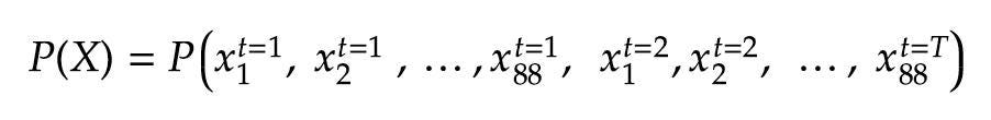
Our overarching goal is to produce a model that efficiently approximates the data generating distribution, P(X). This distribution is a function that maps any sequence of piano notes, X, to a real number ranging between 0 and 1. In essence, P(X) assigns larger values to sequences that are more likely to have been created by skilled human composers. For example, if X¹ is a composition consisting of 200 hours of randomly selected notes, and X² is a Mozart sonata, then P(X¹) < P(X²). Further, P(X¹) will be very near zero.

我们的总体目标是建立一个有效地近似数据生成分布P(X)的模型。 这种分布是一种将钢琴音符X的任何序列映射到介于0和1之间的实数的功能。实质上，P(X)将更大的值分配给更有可能由熟练的人类作曲家创建的序列。 例如，如果X 1是由200小时随机选择的音符组成的组成，而X 2是莫扎特奏鸣曲，则P(X 1)＜P(X 2)。 此外，P(X 1)将非常接近零。

In practice, the distribution P(X) can never be exactly determined, as this would require gathering all the human composers that could ever exist into a room and making them write piano music for all of eternity. However, the same incompleteness exists for simpler data generating distributions. For example, exactly determining the distribution of human heights requires all possible humans to exist and be measured, but this doesn’t stop us from defining and approximating such a distribution. In this sense, the P(X) defined above is a useful mathematical abstraction that encompasses all possible factors determining how piano music is generated.

在实践中，永远无法精确确定分布P(X)，因为这将需要将所有可能存在的人类作曲家聚集到一个房间里，并使他们永远写钢琴音乐。 但是，对于更简单的数据生成分布，存在相同的不完整性。 例如，精确确定人的身高分布要求所有可能的人都存在并被测量，但这并不能阻止我们定义和近似这种高度分布。 从这个意义上讲，上面定义的P(X)是有用的数学抽象，它包含确定钢琴音乐产生方式的所有可能因素。

If we estimate P(X) well enough with a model, we can use that model to stochastically sample new, realistic compositions that have never been heard before. This definition is still a little abstract, so let’s apply some sensible approximations to make the estimation of P(X) more tractable.

如果我们用模型足够好地估计P(X)，则可以使用该模型随机采样以前从未听说过的新的，现实的构图。 这个定义仍然有点抽象，因此让我们应用一些合理的近似值，以使P(X)的估计更易处理。

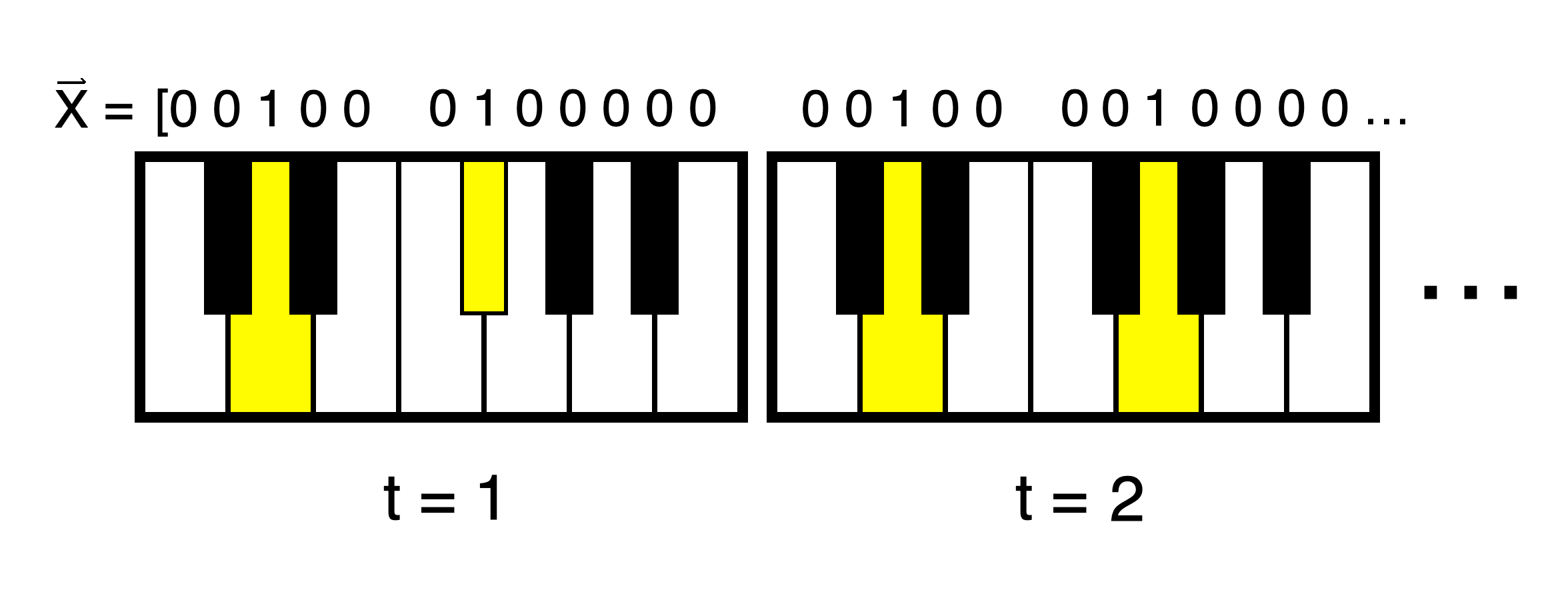
Data Encoding: We need to encode piano music in a way that a computer can understand. To do this, we will represent a piano composition as a variable-length time series of binary states, each state tracking whether or not a given note on the keyboard is being pressed down by a finger during a time step:

数据编码：我们需要以一种计算机可以理解的方式对钢琴音乐进行编码。 为此，我们将钢琴作品表示为二进制状态的可变长度时间序列，每个状态跟踪在某个时间步中是否用手指按下了键盘上的给定音符：

The data processing inequality tells us that information can only ever be lost when we process information,² and our chosen method of encoding of piano music is no exception. There are two ways information loss can happen in this case. First, resolution in the time direction must be limited by making the time steps finite. Luckily, a rather large step size of 0.02 seconds still leads to negligible reduction in music quality. Second, we do not represent the velocity with which keys are being pressed, and thus, musical dynamics are lost.

数据处理的不平等告诉我们，信息只有在我们处理信息时才会丢失，²而且我们选择的钢琴音乐编码方法也不例外。 在这种情况下，有两种方法可以造成信息丢失。 首先，必须通过限制时间步长来限制时间方向的分辨率。 幸运的是，0.02秒的较大步长仍然导致音乐质量的下降可忽略不计。 其次，我们不代表按下键的速度，因此失去了音乐动力。

Despite significant approximations, this encoding method captures much of the underlying information in a concise and machine-friendly form. This is because a piano is effectively a big mechanical finite state machine. Efficiently encoding the music of other, more nuanced instruments, such as a guitar or a flute, would likely be much harder.

尽管有很大的近似值，但是这种编码方法以简洁且机器友好的形式捕获了很多基础信息。 这是因为钢琴实际上是大型的机械有限状态机。 有效地编码其他更细微的乐器(例如吉他或长笛)的音乐可能会困难得多。

Now that we have an encoding scheme, we can represent the data generating distribution in a more concrete form:

现在我们有了编码方案，我们可以用更具体的形式表示数据生成分布：

As an example, at t=1, x₁ = 1 if the first note on a piano is pressed down during the first time step.

例如，如果在第一个时间步中按下钢琴上的第一个音符，则在t = 1时， x₁ = 1。

Factorizing the Distribution: Another simplification involves factorizing the joint probability distribution in (1) using the chain rule of probability:

分解分布：另一个简化方法是使用概率链规则将(1)中的联合概率分布分解：

Similar to n-gram language models, we can make a Markov assumption that notes having occurred more than N time steps in the past have no impact on whether a note at time t=n is pressed. This allows us to rewrite each of the factors in (2) using, at most, the last N note states:

类似于n- gram语言模型，我们可以做出马尔可夫假设，即过去发生的时间超过N个时间步长的音符对是否按下时间t = n的音符没有影响。 这使我们最多使用最后N个音符状态来重写(2)中的每个因子：

Note that, at the beginning of a song, the note history can be padded with up to N zeros so that there is always a history of at least N notes. Also, note that N must be in the hundreds of time steps (many seconds of history) for this approximation to work well for piano music. We will later see that N is determined by the receptive field of our model, and is a key determinant in the quality of performances.

请注意，在一首歌曲的开头，音符历史可以用N个零填充，因此总会有至少N个音符的历史。 另外，请注意， N必须处于数百个时间步长(历史记录的许多秒)中，此近似值才能很好地适用于钢琴音乐。 稍后我们将看到N由我们模型的接受域确定，并且是性能质量的关键决定因素。

At last, we have covered enough mathematical background to rigorously define the task of this project: Using a dataset of encoded sequences of real piano music, train an estimator p̂ that gives the next note’s probability of being pressed down given the last N note states. We can then repeatedly sample the next note using p̂, updating the note history after each sampling, auto-regressively creating an entirely new composition.

最后，我们涵盖了足够的数学背景，可以严格地定义该项目的任务： 使用真实钢琴音乐的编码序列数据集，训练一个估计器p̂，给出给定最后N个音符状态下一个音符被按下的可能性。 然后，我们可以使用p̂重复采样下一个音符，在每次采样后更新音符历史，自动回归创建一个全新的合成。

In this project, our estimator p̂ will be a fully convolutional deep neural network. But, before we can talk about model architectures or training, we need to collect some data.

在这个项目中，我们的估计量p̂将是一个完全卷积的深度神经网络。 但是，在我们谈论模型架构或培训之前，我们需要收集一些数据。

经验 (Experience)

The data our model sees during training will largely determine the quality and style of its generated music. Further, the joint probability distribution we are trying to estimate is very high-dimensional and is prone to issues of data sparsity. This can be overcome by using sufficiently large amounts of training data and appropriate model selection. Regarding the former, piano music is quite easy to collect and preprocess en masse for two reasons.

我们的模型在训练过程中看到的数据将在很大程度上决定其生成的音乐的质量和风格。 此外，我们试图估计的联合概率分布具有很高的维数，并且容易出现数据稀疏的问题。 这可以通过使用足够大量的训练数据和适当的模型选择来克服。 对于前者，钢琴音乐是很容易收集和预处理集体有两个原因。

First, there is a preponderance of piano music on the internet in the form of MIDI files. These files are essentially sequences of piano key states, and minimal preprocessing is needed to get to the encoding we desire for our training data. Second, the task we are trying to accomplish is self-supervised learning, in which our target labels can be automatically generated from the data without manual labeling:

首先，互联网上以MIDI文件的形式盛行钢琴音乐。 这些文件实质上是钢琴键状态的序列，并且需要最少的预处理才能获得我们期望的训练数据编码。 其次，我们要完成的任务是自我监督学习 ，其中可以从数据中自动生成目标标签，而无需手动标签：

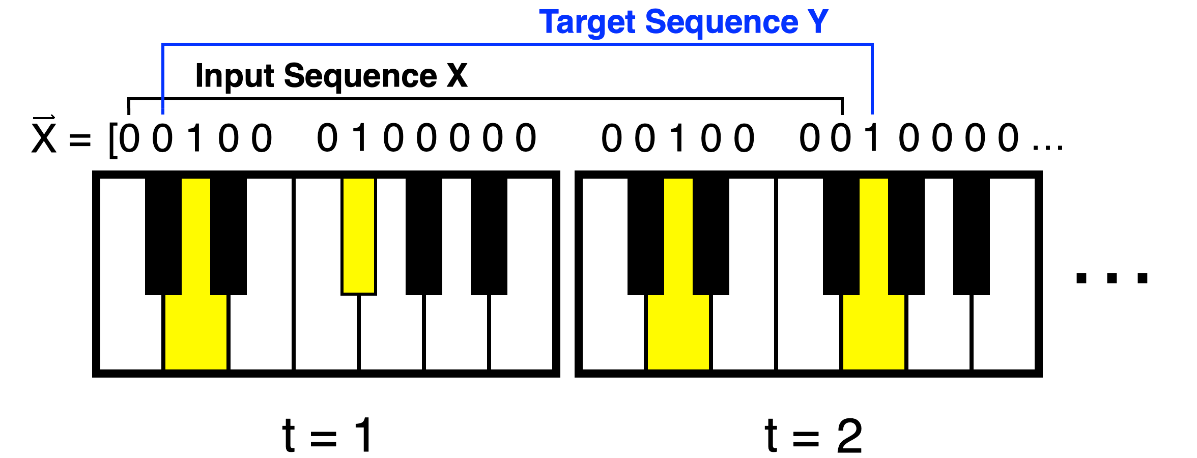
Figure 2 shows how training instances for this task are collected. First, a sequence of binary key states is selected from a song. Then, these states are split into two sub-sequences; an input sequence and then a target sequence of equal size, but with indices shifted forward by one note. All said and done, building our dataset is as simple as downloading quality piano midi files from the internet and manipulating arrays.

图2显示了如何收集此任务的训练实例。 首先，从一首歌曲中选择一系列二进制键状态。 然后，将这些状态分为两个子序列。 一个输入序列，然后是一个大小相等的目标序列，但索引向前移动一个音符。 综上所述，构建我们的数据集就像从互联网上下载高质量的钢琴midi文件并处理数组一样简单。

It’s important to note that the styles of music we include in our training set will largely determine the subspace of the data generating distribution, P(X), that we end up estimating. If we feed the model sequences of Bach and Mozart, it will obviously not learn to generate the jazz music of Thelonious Monk. Due to data collection considerations, I focus on input data from the most famous classical composers, including Bach, Chopin, Mozart, and Beethoven. However, extending this work to different styles of piano music would only require augmenting the dataset with representative examples of these additional styles.

重要的是要注意，我们包含在训练集中的音乐风格将在很大程度上决定我们最终估计的数据生成分布P(X)的子空间。 如果我们输入巴赫(Bach)和莫扎特(Mozart)的模型序列，则显然不会学会产生Thelonious Monk的爵士音乐。 由于数据收集方面的考虑，我将重点放在来自最著名的古典作曲家(包括巴赫，肖邦，莫扎特和贝多芬)的输入数据上。 但是，将这项工作扩展到不同风格的钢琴音乐仅需要使用这些其他风格的代表性示例来扩充数据集。

绩效考核 (Performance Measures)

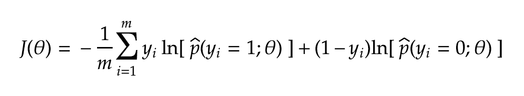
PianoNet is essentially a self-supervised binary classifier that is called repeatedly to predict whether the next key state is up or down. For any probabilistic binary classifier, we can maximize the model’s predicted likelihood of the dataset by minimizing Cross-Entropy loss over the training data:

PianoNet本质上是一个自我监督的二进制分类器，可反复调用以预测下一个键状态是向上还是向下。 对于任何概率二元分类器，我们可以通过最小化训练数据上的交叉熵损失来最大化模型对数据集的预测可能性：

During training, our model is fed long sequences of note-state inputs and targets sampled from human-composed piano music. At each training step, the model uses a finite note history to predict the probability of the next piano key state being pressed. The model will be strongly penalized according to (4) if the predicted probability is close to zero when the true key state is pressed down, or if the predicted probability is close to one when the true key state is not pressed.

在训练过程中，我们的模型会馈入较长的音符状态输入和从人工钢琴音乐采样的目标。 在每个训练步骤中，模型都会使用有限的音符历史记录来预测下一个钢琴键状态被按下的可能性。 如果在按下真实键状态时预测概率接近于零，或者在未按下真实键状态时预测概率接近于一，则将根据(4)对模型进行严厉惩罚。

There is a potential problem with this loss function. Our ultimate goal is not to create a model that predicts a single next note based on past notes in a human-created composition, but rather to create extended sequences of notes based on a history of notes that the model itself generated. In this sense, we are making a very strong assumption: As a model improves at predicting the next piano note’s state when given a history of human-generated note states, it will also generally improve at generating extended performances auto-regressively, using its own output as the note history.

此损失函数存在潜在的问题。 我们的最终目标不是创建一个模型，该模型根据人为组成中的过去音符来预测单个下一个音符，而是根据模型本身生成的音符历史来创建音符的扩展序列。 从这个意义上讲，我们做出了一个非常有力的假设：当给定人类生成的音符状态的历史记录时，随着模型在预测下一个钢琴音符的状态方面的改进，它通常也会在使用自己的音色自动回归生成扩展演奏方面得到改进输出为音符历史。

It turns out, this assumption does not always hold, as models with relatively low validation losses can still sound very unmusical when generating performances. Below, I show that this assumption does not apply to shallow networks, but for sufficiently deep networks, it applies well in practice.

事实证明，这种假设并不总是固定，如用相对较低的验证损失模型可以生成演出的时候依然声音非常非音乐。 下面，我表明该假设不适用于浅层网络，但对于足够深的网络，它在实践中适用。

模型架构 (Model Architecture)

We now know how to define the task and can collect large amounts of properly encoded data, but what model should we train on the data to perform better at the task of piano composition? As a good starting point, our model should have a few properties that should improve its ability to generalize to unseen data:

现在，我们知道了如何定义任务并可以收集大量正确编码的数据，但是我们应该在数据上训练哪种模型才能更好地完成钢琴演奏任务？ 作为一个良好的起点，我们的模型应该具有一些属性，这些属性应该可以提高其泛化为看不见的数据的能力：

• The model should be invariant to transpositions in key, that is, moving pressed notes up or down in pitch by a fixed number of keys: To a good approximation, a Mozart Sonata starting with a C major chord should have the same relative note distribution as a Sonata starting with a G major chord. The keys are not entirely symmetric to transposition, but the relative frequencies of the tones is what largely determines the musical semantics of a composition. This phenomenon is why a band can cover Tom Petty’s Free Falling in a key that’s a little more comfortable for the lead vocalist without the audience noticing.

  该模型应不变于琴键的移调，也就是说，按固定数量的琴键将按下的音符在音高上上下移动：为了获得良好的近似，以C大和弦开头的Mozart奏鸣曲的相对音符分布应与以G大调和弦开头的奏鸣曲 琴键与移调并不完全对称，但是音调的相对频率在很大程度上决定了乐曲的音乐语义。 这就是为什么乐队可以在不引起观众注意的情况下用主键歌手更轻松一点的方式覆盖Tom Petty的《 Free Falling 》的原因。

• The model should be invariant to small changes in tempo: If a song is played 2% faster or slower, this should not impact the distribution of next notes very much. It turns out that we can’t impose this invariance directly, but we can teach the model tempo invariance by using data augmentation.

  该模型应该对速度的微小变化保持不变：如果将歌曲的播放速度提高或降低2％，则这不会严重影响下一音符的分布。 事实证明，我们不能直接施加这种不变性，但可以通过使用数据增强来教导模型速度不变性。

• The model should not reduce input resolution as data flows through the network: The distribution of future notes can be very sensitive to high-resolution nuances in the music, especially rhythmic variations in the time direction, so we shouldn’t destroy this information. In this respect, it’s assumed that techniques like pooling would hurt model performance.

  当数据流经网络时，该模型不应降低输入分辨率：将来音符的分布可能对音乐中的高分辨率细微差别非常敏感，尤其是时间方向上的节奏变化，因此我们不应该破坏此信息。 在这方面，假设池化之类的技术会损害模型性能。

• The number of model parameters should scale well with size of the receptive field: The total receptive field is the size of the model’s input. The larger this is, the more note history that can be used to influence the probability of future notes. In piano music, this must be at least a few seconds long. The number of model parameters should remain in the millions or fewer for a few-second receptive field.

  模型参数的数量应与接受区域的大小很好地缩放：总接受区域是模型输入的大小。 此值越大，可用于影响未来票据概率的票据历史记录就越多。 在钢琴音乐中，该时间必须至少为几秒钟。 对于几秒钟的接收字段，模型参数的数量应保持在数百万或更少。

Fully convolutional neural networks composed of stacked dilated convolution layers are a simple but effective choice for satisfying the above properties. The dilated convolution is like a traditional convolution, except that there may be a gap of length one or more between kernel inputs. See this TDS blog post for a more detailed overview of dilated convolutions, although we’re using 1D convolutions in this case, not 2D.

由堆叠的膨胀卷积层组成的全卷积神经网络是满足上述特性的简单但有效的选择。 扩张卷积类似于传统卷积，不同之处在于内核输入之间可能存在一个或多个长度的间隙。 请参阅此TDS博客文章 ，以详细了解膨胀卷积，尽管在这种情况下，我们使用的是1D卷积，而不是2D。

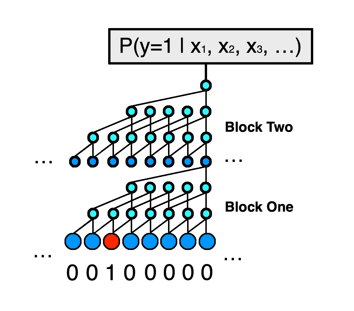
Similar to the approach used in the WaveNet paper,¹ we will construct our model using an exponentially growing dilation rate within each ‘block’, and stack multiple blocks to create the full network. Below is example Tensorflow code for constructing a model with two blocks, each block having seven layers. The network gets wider and wider throughout, such that the second block has many more filters in each layer than the first. Finally, the model ends with a single filter whose output is run through a sigmoid activation, and this output will be the predicted probability that the next note state is one.

与WaveNet论文中使用的方法类似，¹我们将使用每个“块”内的指数增长速率来构建模型，并堆叠多个块以创建完整的网络。 下面是示例Tensorflow代码，用于构建具有两个块的模型，每个块有七个层。 网络在整个范围内变得越来越宽，因此第二个块在每个层中的过滤器比第一个块多。 最后，模型以单个滤波器结束，该滤波器的输出通过S型激活，并且该输出将是下一个音符状态为1的预测概率。

from tensorflow.keras.layers import Input, Conv1D, Activation
from tensorflow.keras.models import Model
filter_counts = [
    [4,  8,  12, 16, 20, 24, 28], # block one's filter counts[32, 36, 38, 42, 46, 50, 54], # block two's filter counts]
inputs = Input(shape=(None, 1)) # None allows variable input lengthsconv = inputs
for block_idx in range(0, len(filter_counts)):
    block_filter_counts = filter_counts[block_idx]
    for i in range(0, len(block_filter_counts)):
        filter_count = block_filter_counts[i]
        dilation_rate = 2**i # exponentially growing receptive field        conv = Conv1D(filters=filter_count, kernel_size=2,
                      strides=1, dilation_rate=dilation_rate,
                      padding='valid')(conv)
        conv = Activation('elu')(conv)
outputs = Conv1D(filters=1, kernel_size=1, strides=1,
                 dilation_rate=1, padding='valid')(conv)
outputs = Activation('sigmoid')(outputs)
model = Model(inputs=inputs, outputs=outputs)

The line dilation_rate = 2**i causes the dilation rate in each block to start at one (like a conventional convolution with kernel size two), then exponentially increase with each subsequent layer in the block. Once the second block begins, this dilation rate resets to size one, and starts increasing exponentially as before.

线dilation_rate = 2**i使每个块中的膨胀率从1开始(就像内核大小为2的常规卷积一样)，然后随该块中的每个后续层以指数方式增加。 一旦第二个块开始，该膨胀率将重置为大小1，并且像以前一样开始呈指数增长。

We could have let the dilation rate continue to increase exponentially without ever resetting, but this would cause the receptive field to grow too rapidly per model depth. We also do not have to increase the number of filters with each new layer. We could instead let the filter count of each layer always be equal to some large number, like 64. However, while experimenting, I found that starting with a small number of filters and slowly increasing the count results in a more statistically efficient model. Figure 3 shows a schematic model with two blocks:

我们本来可以让扩张率持续指数增长而无需重置，但这会导致每个模型深度的接收场增长过快。 我们也不必增加每个新层的过滤器数量。 相反，我们可以让每层的过滤器数量始终等于某个较大的数量，例如64。但是，在进行实验时，我发现从少量的过滤器开始并逐渐增加计数会导致统计上更有效的模型。 图3显示了具有两个模块的示意图模型：

A final note is required on the padding='valid' argument of each Conv1D layer instantiation. We want our model input to only ever see notes that occurred before the current predicted note - otherwise we would be allowing future information that will not be present at inference time to leak into our predictions. We also do not want to pad an input sequence of notes with zeros (silence). Input sequences may start in the middle of a song, and padding with silence would create an artificial input state where silence is suddenly interrupted by an internal song fragment. The ‘valid’ setting pads the sequences in a way that satisfies the above two requirements.

在每个Conv1D层实例化的padding='valid'参数上需要最后说明。 我们希望我们的模型输入只看到在当前预测音符之前出现的音符-否则，我们将允许在推断时不出现的未来信息泄漏到我们的预测中。 我们也不想在输入的音符序列上填充零(静音)。 输入序列可以从歌曲的中间开始，并且用静音填充会创建人为的输入状态，其中静音会被内部歌曲片段突然打断。 “有效”设置以满足上述两个要求的方式填充序列。

培训技巧和窍门 (Tips and Tricks to Training)

Although it’s easy to procure a large dataset, and the model architectures we’ve discussed are rather simple to construct, training a model that produces realistic music is still an art. Here are some tips to help you to overcome many challenges I was faced with.

尽管获取大型数据集很容易，而且我们已经讨论过的模型体系结构很容易构建，但是训练产生逼真的音乐的模型仍然是一门艺术。 这里有一些技巧可以帮助您克服我所面临的许多挑战。

深度的重要性 (The Importance of Depth)

When I began training models, I started with single-block shallow network architectures, having around 15 layers, with large numbers of weights per layer. Although the validation loss showed that these models were learning from the data and not overfitting, I was dismayed to hear performances like the following:

当我开始训练模型时，我从大约15层的单块浅层网络体系结构开始，每层具有大量权重。 尽管验证损失表明这些模型正在从数据中学习而不是过拟合，但我还是很沮丧地听到如下性能：

演示地址

The shallow network’s performance starts somewhat musically, but as it gets farther and farther from the human-generated seed, it eventually devolves into chaos, eventually giving way to mostly silence.

浅层网络的演奏在音乐上有些开始，但是随着它离人类产生的种子越来越远，它最终演变成混乱，最终让位于大部分沉默。

Surprisingly, when I increased network depth by adding more blocks, but held the number of parameters constant, the performance quality increased dramatically even when validation loss did not decrease:

出人意料的是，当我通过添加更多块来增加网络深度，但保持参数数量不变时，即使验证损失没有减少，性能质量也显着提高：

演示地址

The shallow and deep networks that generated the performances above have nearly the same loss on the validation set, yet the deep network is able to form coherent musical phrases, while the shallow network is…avant-garde. Note that the above two networks are relatively small with narrow receptive fields of 2.6 seconds and 10–40 layers. The more advanced models shown at the beginning of this post have closer to 100 layers and a receptive field of almost 10 seconds. Also, these results are not random. I’ve listened to many minutes of music from both the shallow and deep model using many different seeds, and the pattern remains consistent.

产生上述性能的浅层和深层网络在验证集上损失几乎相同 ，但是深层网络能够形成连贯的音乐短语，而浅层网络则是…… 前卫的 。 请注意，以上两个网络相对较小，具有2.6秒的窄接收场和10-40层。 在本文开头显示的更高级的模型具有接近100层和近10秒的接收范围。 同样，这些结果也不是随机的。 我已经使用许多不同的种子从浅层模型和深层模型中听了很多分钟的音乐，并且模式保持一致。

Why doesn’t validation loss tell the whole story? Remember that the loss we’re using measures the model’s ability to predict the next note given a large history of human-generated notes. This will relate to, but not entirely capture, a model’s ability to auto-regress a clean performance using its own generated note history for long stretches without devolving into a space within P(X) for which it has not been given representative training data. The Cross-Entropy loss given in (4) is an intrinsic measure that is convenient for training, but the subjective quality of the performances is the true extrinsic measure.

为什么验证损失不能说明全部情况？ 请记住，鉴于人类产生的音符已有很长的历史，我们使用的损失量度了模型预测下一个音符的能力。 这将涉及(但不完全捕获)模型使用其 自身生成的音符历史记录进行长时间拉伸而自动回归清洁演奏的能力，而不会移入P(X)内尚未获得代表性训练数据的空间。 (4)中给出的交叉熵损失是一种便于训练的内在度量，但是表演的主观质量是真正的外在度量。

I have supported why low validation loss doesn’t imply a good sounding performance, but why does adding depth to our network tend to improve musicality for the same loss? It’s likely that statistical efficiency is the determining factor here. Deep-and-thin convolutional neural networks likely represent the family of functions we are trying to estimate more efficiently than their shallow-and-wide counterparts. The process of composing music, like many human tasks, seems to be better represented as a series of many compositions of simpler functions, as opposed to that of a few relatively complex functions. It is likely that the shallow networks are ‘memorizing’ common patterns in the note history, while the deeper networks are encoding these patterns into more meaningful representations that vary less with small variations in the input.

我已经支持了为什么低的验证损失并不意味着良好的发声性能，但是为什么在相同的损失下增加网络的深度却可以改善音乐性呢？ 统计效率可能是决定因素。 薄层卷积神经网络可能代表我们试图比其浅层和宽层同行更有效地估计的函数族。 就像许多人工任务一样，音乐创作的过程似乎可以更好地表示为一系列由许多较简单的功能组成，而不是一些相对复杂的功能。 浅层网络可能会“记住”音符历史记录中的常见模式，而较深层网络会将这些模式编码为更有意义的表示，而输入中的细微变化则变化较小。

There is one final heuristic regarding depth that I’ve found improves performance and reduces training time. The receptive field of each additional block should shrink by a factor of two relative to the last block. This entails each subsequent block having one fewer layer than the last. This greatly reduces the number of convolution operations, as the widest layers (those near the output layer) have the smallest receptive fields. At the same time, the overall receptive field of the model is not greatly affected if the first layers have rather large receptive fields.

我发现关于深度的最后一种启发式方法可以提高性能并减少训练时间。 每个附加块的接收场应相对于最后一个块缩小两倍。 这使得每个随后的块比最后一个块少一层。 由于最宽的层(靠近输出层的层)具有最小的接收场，因此这大大减少了卷积运算的次数。 同时，如果第一层具有较大的接收场，则不会大大影响模型的整体接收场。

我应该训练多长时间？ 长一点 (How Long Should I Train? Longer.)

Each additional block added to the network adds significant depth — around ten layers each block. Thus, getting these deep networks to train can quickly be tricky. To combat exploding gradients during training, the learning rate needs to be rather small, usually around 0.0001, which means the model must train for many more steps before it converges on a good solution.

添加到网络中的每个其他块都会增加可观的深度-每个块大约十层。 因此，快速训练这些深度网络可能很棘手。 为了在训练过程中应对爆炸梯度，学习率必须很小，通常约为0.0001，这意味着模型必须训练更多的步骤才能收敛到良好的解决方案。

There is a silver lining, however. Because we have access to so much data (billions of note states), it’s difficult for a modest-sized model with a million or so parameters to overfit the dataset. This effectively means that, the longer you let your model train, the better it will sound. The validation loss will decrease less and less as training progresses, but the model continues to learn extremely important elements of the music late into training.

但是，有一线希望。 因为我们可以访问如此多的数据(数十亿个音符状态)，所以具有一百万个左右参数的适度大小的模型很难拟合数据集。 这实际上意味着，让模型训练的时间越长，声音越好。 随着训练的进行，验证损失将越来越少，但是该模型在训练后期仍会继续学习音乐中极为重要的元素。

To prove how important it is to let the model train sufficiently long, here is a set of mini performances showing how a given model learns as training progresses. Each mini performance has the same human-composed seed, consisting of a snippet of Beethoven’s Für Elise. With each repetition, the model is given more and more training time before it is asked to complete the seed:

为了证明让模型训练足够长的时间非常重要，这是一组微型表演，展示了给定模型如何随着训练的进行而学习。 每个迷你演出都有相同的人为组成的种子，其中包括贝多芬的《 FürElise》片段。 瓦特 i个每次重复，模型给出之前，要求完成的种子越来越多的培训时间：

演示地址

We see that, it’s not until the last 20% of training wall-time that the model produces musically sensible phrasings.

我们看到，直到训练壁挂时间的最后20％时，模型才产生音乐上合理的用语。

To speed up training a bit, I often start with a batch size of one and slowly increase it to 32. This encourages exploration across the parameter space and limits the amount of compute resources required. We can get away with an initial batch size of one because each individual training sample can contain hundreds of predictions across a song segment (see the input and target sequences in Figure 2).

为了加快培训速度，我通常从批处理大小为1开始，然后逐渐将其增加为32。这鼓励在参数空间上进行探索，并限制了所需的计算资源量。 最初的批量大小为1可以避免，因为每个单独的训练样本可以在歌曲片段中包含数百个预测(请参见图2中的输入和目标序列)。

战略偏差初始化 (Strategic Bias Initialization)

Most of the time, a piano key is not being pressed. Only the most experimental artists will ever press more than a few keys at any time step. This makes it very important to set the bias correctly in our output layer:

大多数情况下，不会按下钢琴键。 在任何时候，只有大多数实验性艺术家会按下多个键。 这使得在我们的输出层中正确设置偏差非常重要：

output_bias_init = tensorflow.keras.initializers.Constant(-3.2)outputs = Conv1D(filters=1, kernel_size=1, strides=1,
                 dilation_rate=1, padding='valid',
                 bias_initializer=output_bias_init)(conv)outputs = Activation('sigmoid')(outputs)

By setting bias to -3.2, our model predicts the correct base rate of notes being pressed on average (around 0.04) from the outset. The model no longer has to spend many training steps figuring out that piano keys simply aren’t pressed that often. This removes the hockey stick learning curve and speeds up training a bit.

通过将偏差设置为-3.2，我们的模型可以从一开始就预测平均平均正确的基准汇率(大约0.04)。 该模型不再需要花费很多训练步骤就可以确定钢琴琴键不会被频繁按下。 这消除了曲棍球棒的学习曲线，并加快了训练速度。

数据扩充 (Data Augmentation)

In the same way that rotating and scaling images can help models generalize better in computer vision tasks, we can stretch and compress our 1D sequences of piano notes by a few percent to further augment the training data. The idea is that a given piano piece could have been played a little faster or a little slower without altering its chance of being sampled from the data generating distribution. This helps considerably in the fight against data sparsity, and it also helps the model learn to be invariant to small changes in tempo. I usually create five clones of each input song, stretched randomly between 15% slower and 15% faster.

就像旋转和缩放图像可以帮助模型更好地推广计算机视觉任务一样，我们可以将钢琴音符的一维序列拉伸和压缩几个百分点，以进一步增强训练数据。 这个想法是，给定的钢琴演奏本来可以快一点或慢一点，而不会改变从数据生成分布中采样的机会。 这在对抗数据稀疏性方面有很大帮助，并且还帮助模型学习了速度的微小变化是不变的。 我通常为每个输入歌曲创建五个克隆，它们在15％到15％的速度之间随机拉伸。

安全地创建验证数据集 (Safely Creating the Validation Dataset)

We should not sample random segments of all songs when building the training and validation sets. Piano songs often repeat entire sections, so if we use a random sampling approach, we likely would end up inadvertently training on the validation set.

构建训练和验证集时，我们不应该对所有歌曲的随机片段进行采样。 钢琴歌曲通常会重复整个部分，因此，如果我们使用随机采样方法，最终可能会无意间对验证集进行训练。

To avoid this, we must ensure that the training and validation sets are assigned entirely distinct songs, before splitting them into sample segments. As long as the number of songs sampled from each composer is in the hundreds, we will still will get a reasonable estimate of the model’s generalization error on unseen music.

为避免这种情况，我们必须确保在将训练和验证集分成样本片段之前，将它们分配给完全不同的歌曲。 只要每个作曲家采样的歌曲数为数百，我们仍将对模型在看不见的音乐上的泛化误差做出合理的估计。

作曲家与熵 (Composers and Entropy)

On average, different composers will have higher or lower musical entropies. That is, composers’ compositions will be more or less unpredictable, in that there will be more or less uncertainty in what note may follow the previous notes. In general, earlier composers, such as Bach or Haydn, will have lower uncertainty in their data generating distributions, while later composers, such as Prokofiev or Ravel, will have many more possible notes given a history of notes.

平均而言，不同的作曲家会具有更高或更低的音乐熵。 就是说，作曲家的创作或多或少是不可预测的，因为前一个音符后面的音符或多或少具有不确定性。 通常，较早的作曲家，如巴赫(Bach)或海顿(Haydn)，在数据生成分布方面的不确定性较低，而较晚的作曲家，如普罗科菲耶夫(Prokofiev)或拉威尔(Ravel)，由于音符的历史，将有更多可能的音符。

Due to this varying degree of entropy, don’t be surprised if more model capacity, training time, and/or training data is required for your model to reproduce more unpredictable styles. In my experience, the models described in this post often can easily replicate Bach’s works with a hundred songs, while getting a model to produce compelling Chopin music seems to take much more input data.

由于熵的变化程度不同，如果模型需要更多的模型容量，训练时间和/或训练数据来再现更多不可预测的样式，请不要感到惊讶。 以我的经验，这篇文章中描述的模型通常可以轻松地复制巴赫的作品与上百首歌曲，而让模型产生引人入胜的肖邦音乐似乎需要更多的输入数据。

使用训练有素的模型来产生表现 (Generating Performances Using Trained Models)

天真的模型推断 (Naive Model Inference)

Once you have a trained model, you’ll want to use it to generate new compositions. To generate a performance, we start with an input seed equal in length to the model’s receptive field. This seed can be part of a song written by a human, or simply silence. We can then call the model.predict on this input seed to generate a probability that the state of the first key in the next time step is pressed down. If this prediction is 0.01, then we will sample the next key being pressed down with 1% probability.

拥有训练有素的模型后，您将需要使用它来生成新的合成。 为了产生性能，我们从输入种子开始，该种子的长度等于模型的接受场。 该种子可以是人类创作的歌曲的一部分，也可以只是沉默。 然后，我们可以在此输入种子上调用model.predict ，以产生下一个步骤中第一个键的状态被按下的概率。 如果此预测为0.01，那么我们将以1％的概率采样下一个按下的键。

If we drop the first note from the input seed, and add the model’s last sampled note state to the end, then we once again have an input vector equal in length to the model’s receptive field. We can use the new input to generate yet another key state, this time using the model’s last output as part of the input. Finally, we can repeat this process indefinitely, at some point the input being entirely generated by our model. This is the core idea behind autoregression.

如果我们从输入种子中删除第一个音符，并将模型的最后一个采样音符状态添加到末尾，那么我们将再次得到一个输入矢量，其长度等于模型的接收场。 我们可以使用新输入来生成另一个键状态，这次使用模型的最后输出作为输入的一部分。 最后，我们可以无限期地重复此过程，有时输入完全由我们的模型生成。 这是自回归背后的核心思想。

快速WaveNet生成算法 (Fast WaveNet Generation Algorithm)

Although the above approach will work just fine, it could take hours to generate a minute of music. This is because each model.predict(input) call requires a very large number of successive convolution operations to compute the final output, and the compute time scales poorly with model depth.

尽管上述方法可以很好地工作，但生成一分钟的音乐可能要花费数小时。 这是因为每个model.predict(input)调用都需要大量连续的卷积运算来计算最终输出，并且计算时间随模型深度的变化而model.predict(input) 。

It turns out we can speed up these calculations significantly if we store some information from past convolution operations in a queue. This is the idea behind the Fast Wavenet Generation Algorithm. How this algorithm works is beyond the scope of this post, but rest assured, I’ve implemented a pure Python version in the PianoNet package described in more detail below. If you use this package, even with a very large network containing millions of parameters, generating a minute of piano music will take on the order of five minutes, rather than hours.

事实证明，如果我们将过去卷积操作中的某些信息存储在队列中，则可以大大加快这些计算的速度。 这就是快速波网生成算法的思想。 该算法的工作原理超出了本文的范围，但是请放心，我已经在PianoNet包中实现了一个纯Python版本，下面将对此进行详细介绍。 如果使用此程序包，即使在包含数百万个参数的超大型网络中，产生一分钟的钢琴音乐也要花费五分钟的时间，而不是几小时。

边缘厌恶 (Edge Aversion)

One last detail regarding performance generation involves constraining the model from drifting. Because our architecture is invariant with respect to key changes, it does not encode which octave a key state is in. This means the model treats all octaves on the keyboard as equally likely, and can drift toward the edges of the piano key states. We don’t want this to happen, because composers tend to keep the pressed keys closer to the middle of the piano.

关于性能生成的最后一个细节涉及限制模型的漂移。 因为我们的体系结构在键更改方面是不变的，所以不会对键状态所在的八度进行编码。这意味着模型将键盘上的所有八度均等地对待，并且可能会移向钢琴键状态的边缘。 我们不希望这种情况发生，因为作曲家倾向于使按下的琴键更靠近钢琴的中央。

To combat this drift in the simplest way possible, I’ve applied what I call edge aversion. This approach is a way to bias the model away from the edges during performances without altering the model’s output distribution too much. In essence, edge aversion enforces that the very highest and very lowest notes on a piano keyboard are only played when the model predicts a very high probability. For example, if the model predicts that the highest key on the piano will be pressed with a probability of 0.05, the key will still never be randomly sampled as pressed.

为了以最简单的方式应对这种漂移，我应用了所谓的边缘厌恶。 这种方法是在执行过程中使模型偏离边缘的一种方法，而不会过多改变模型的输出分布。 本质上，边缘厌恶要求只有在模型预测到非常高的概率时，才会弹奏钢琴键盘上的最高音和最低音。 例如，如果模型预测将以0.05的概率按下钢琴上的最高琴键，则该琴键仍将永远不会在被按下时被随机采样。

使用PianoNet Python软件包 (Using the PianoNet Python Package)

At this point, you may be excited to start training your own models for generating piano music. To make this process as easy as possible, I’ve created PianoNet, a Python package for easily reproducing the work I describe above.

在这一点上，您可能会兴奋地开始训练自己的模型来生成钢琴音乐。 为了使此过程尽可能简单，我创建了PianoNet ，这是一个Python软件包，用于轻松复制我上面描述的工作。

For a full end-to-end tutorial on how to use the package, please see the readme file contained in the linked repo. In the below sections, I’ll briefly talk about the abstractions used for controlling data collection, model training, and performance generation. The basic steps for any workflow are always:

有关如何使用该软件包的完整的端到端教程，请参阅链接的存储库中包含的自述文件。 在以下各节中，我将简要讨论用于控制数据收集，模型训练和性能生成的抽象。 任何工作流程的基本步骤始终是：

• Create training and validation MasterNoteArray files using the pianonet/scripts/master_note_array_creation.py script
  使用pianonet / scripts / master_note_array_creation.py脚本创建培训和验证MasterNoteArray文件
• Create a directory that holds your calculation and contains a run_description.json file, which specifies the hyperparameters for training and links to the input data files
  创建一个目录来保存您的计算，并包含一个run_description.json文件，该文件指定用于训练的超参数以及指向输入数据文件的链接
• Use the pianonet/scripts/runner.py script to start a run in the same directory
  使用pianonet / scripts / runner.py脚本在同一目录中开始运行

• Once training finishes, use the get_performance method in pianonet/model_inspection/performance_tools.py to generate performances

  培训结束后，请使用pianonet / model_inspection / performance_tools.py中的get_performance方法来生成演奏

收集和预处理数据 (Collecting and Pre-Processing Data)

Step one is to find a handful of midi files containing piano performances in the styles you want the model to learn. The internet is a great place to find free piano midi files from all sorts of composers. Once you’ve collected these files, move them all to a directory of your choosing. I'll assume they’re located at /path/to/midi/ in this example.

第一步是找到一些Midi文件，其中包含您希望模型学习的风格的钢琴演奏。 互联网是查找来自各种作曲家的免费钢琴midi文件的好地方。 收集完这些文件后，将它们全部移到您选择的目录中。 在此示例中，我假设它们位于/path/to/midi/中。

To train models using the PianoNet package, we need to extract all of our midi files into training and validation MasterNoteArray instances saved to disk. A MasterNoteArray object is essentially a 1D array of all input songs concatenated in a way that is amenable to training. We can create a data description json file for generating the MasterNoteArray, such as the following:

要使用PianoNet软件包训练模型，我们需要将所有的midi文件提取到训练和验证保存到磁盘的MasterNoteArray实例中。 MasterNoteArray对象本质上是所有输入歌曲的一维数组，其连接方式适合训练。 我们可以创建一个数据描述json文件来生成MasterNoteArray，如下所示：

{
        
  "file_name_prefix": "dataset_master_note_array",
  "min_key_index": 31,
  "num_keys": 72,
  "resolution": 1.0,
  "end_padding_range_in_seconds": [
    4.0,
    6.0
  ],
  "num_augmentations_per_midi_file": 5,
  "stretch_range": [
    0.85,
    1.15
  ],
  "time_steps_crop_range": [],
  "midi_locator": {
        
    "paths_to_directories_of_midi_files": ["/path/to/midi/"],
    "whitelisted_midi_file_names": []
  },
  "validation_fraction": 0.2
}

Make sure to change the /path/to/midi/ path above to wherever you store your midi files. For more augmentations (stretching of each song), increase the num_augmentations_per_midi_file from five to a larger number.

Make sure to change the /path/to/midi/ path above to wherever you store your midi files. For more augmentations (stretching of each song), increase the num_augmentations_per_midi_file from five to a larger number.

Finally, we can generate our input datasets using the following command:

Finally, we can generate our input datasets using the following command:

python pianonet/scripts/master_note_array_creation.py /path/to/data_description.json /path/to/output/directory

This script will generate two .mna_jl files, one containing the training data, one containing the validation data.

This script will generate two .mna_jl files, one containing the training data, one containing the validation data.

Training Models (Training Models)

Once we have our MasterNoteArray datasets, we can start model training sessions, or runs. Each run sits in its own directory, and has a single run_description.json file describing how the run should be performed:

Once we have our MasterNoteArray datasets, we can start model training sessions, or runs. Each run sits in its own directory, and has a single run_description.json file describing how the run should be performed:

{
        
  "data_description": {
        
    "training_master_note_array_path": "./dataset_train.mna_jl",
    "validation_master_note_array_path": "./dataset_val.mna_jl"
  },
  "model_description": {
        
    "model_path": "",
    "model_initializer": {
        
      "path": "pianonet/scripts/model_generators/basic_convolutional_with_blocks.py",
      "params": {
        
        "filter_increments": [
          [ 4, 4, 4, 4, 4, 4, 4, 4, 4, 4, 4, 4],
          [ 4, 4, 4, 4, 4, 4, 4, 4, 4, 4, 4],
          [ 6, 6, 6, 6, 6, 6, 6, 6, 8, 8],
        ],
        "default_activation": "elu",
        "use_calibrated_output_bias": true
      }
    }
  },
  "training_description": {
        
    "batch_size": 8,
    "num_predicted_time_steps_in_sample": 24,
    "epochs": 10000,
    "checkpoint_frequency_in_steps": 250,
    "fraction_data_each_epoch": 0.1,
    "loss": "binary_crossentropy",
    "optimizer_description": {
        
      "type": "Adam",
      "kwargs": {
        
        "lr": 0.0001,
        "beta_1": 0.9,
        "beta_2": 0.999,
        "epsilon": 1e-07,
        "decay": 0.0
      }
    }
  },
  "validation_description": {
        
    "batch_size": 1,
    "num_predicted_time_steps_in_sample": 512,
    "fraction_data_each_epoch": 1.0
  }
}

It’s important that training_master_note_array_path and validation_master_note_array_path both point to the .mna_jl files you created in the dataset creation step.

It's important that training_master_note_array_path and validation_master_note_array_path both point to the .mna_jl files you created in the dataset creation step.

The model_description parameter describes how the model should be generated. Each list in filter_increments controls a block, with each number representing the increase in filter count for the current layer relative to the previous layer’s filter count. Adding more lists would increase the model capacity by adding depth (more blocks), while increasing the filter increment magnitudes would add width to the model. The rest of the descriptor fields are fairly self-explanatory, and they allow you to control hyperparameters like batch size, how many predicted notes each input sample sequence contains, and arguments of the optimizer. The above numbers all represent sensible defaults.

The model_description parameter describes how the model should be generated. Each list in filter_increments controls a block, with each number representing the increase in filter count for the current layer relative to the previous layer's filter count. Adding more lists would increase the model capacity by adding depth (more blocks), while increasing the filter increment magnitudes would add width to the model. The rest of the descriptor fields are fairly self-explanatory, and they allow you to control hyperparameters like batch size, how many predicted notes each input sample sequence contains, and arguments of the optimizer. The above numbers all represent sensible defaults.

Once you’ve created the run_description.json file and have located it in the run directory, you can start the training using:

Once you've created the run_description.json file and have located it in the run directory, you can start the training using:

python pianonet/scripts/runner.py /path/to/run/directory

This will start a training session in you terminal. To view the output logs for the run, start another terminal in the run directory and use tail -f training_output.txt to see the logs in real time as training progresses.

This will start a training session in you terminal. To view the output logs for the run, start another terminal in the run directory and use tail -f training_output.txt to see the logs in real time as training progresses.

Models will be periodically saved in the models directory within the run path, with files names like 0_trained_model. If training is stopped, it can be restarted using the above command and will start from the last saved model.

Models will be periodically saved in the models directory within the run path, with files names like 0_trained_model . If training is stopped, it can be restarted using the above command and will start from the last saved model.

Generating Performances (Generating Performances)

The last step, once you’ve trained the model sufficiently, is to listen to how it sounds. This involves inputting your trained model’s file path and a seed to the performance tools method. I’ve created a jupyter notebook overviewing how to do this step by step, which can be found at pianonet/examples/pianonet_mini/get_performances.ipynb.

The last step, once you've trained the model sufficiently, is to listen to how it sounds. This involves inputting your trained model's file path and a seed to the performance tools method. I've created a jupyter notebook overviewing how to do this step by step, which can be found at pianonet/examples/pianonet_mini/get_performances.ipynb .

结论 (Conclusions)

Fully convolutional neural networks based on dilated convolutions can successfully generate convincing piano music when trained correctly. These models can be fed raw sequences of notes, are straightforward to build, and can be easy to train with the help of a few tricks. Best of all, they can generate music almost realtime if the Fast-WaveNet algorithm is used. PianoNet is a python package that makes it easy to reproduce all of these features.

Fully convolutional neural networks based on dilated convolutions can successfully generate convincing piano music when trained correctly. These models can be fed raw sequences of notes, are straightforward to build, and can be easy to train with the help of a few tricks. Best of all, they can generate music almost realtime if the Fast-WaveNet algorithm is used. PianoNet is a python package that makes it easy to reproduce all of these features.

Although performances from these fully-convolutional networks sound quite good, they are lacking in some respects compared to the transformer-based architectures mentioned in the introduction. Because fully-convolutional networks are effectively constrained to have receptive fields shorter than twenty seconds, they are incapable of learning song patterns extending beyond this time scale, such as the repeating structure of the sonata form. It’s also difficult for the convolutional models to learn melodic motifs, something that NLP-based transformer models seem to do quite well.

Although performances from these fully-convolutional networks sound quite good, they are lacking in some respects compared to the transformer-based architectures mentioned in the introduction. Because fully-convolutional networks are effectively constrained to have receptive fields shorter than twenty seconds, they are incapable of learning song patterns extending beyond this time scale, such as the repeating structure of the sonata form. It's also difficult for the convolutional models to learn melodic motifs, something that NLP-based transformer models seem to do quite well.

Despite these shortcomings, the fully-convolutional architectures described in this post are relatively simple, easy to work with, and are a quick way to have some fun exploring the possibilities of machine-generated art.

Despite these shortcomings, the fully-convolutional architectures described in this post are relatively simple, easy to work with, and are a quick way to have some fun exploring the possibilities of machine-generated art.