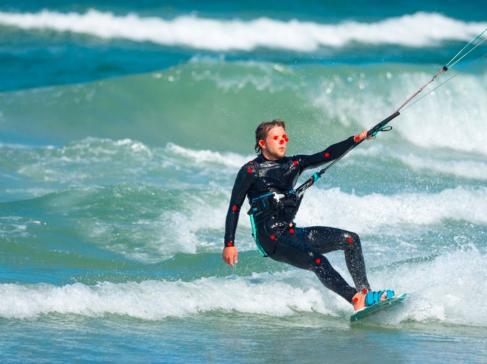
默认情况下，PyTorch 提供了一个 Keypoint RCNN 模型，该模型经过预训练以检测人体的 17 个关键点（鼻子、眼睛、耳朵、肩膀、肘部、手腕、臀部、膝盖和脚踝）。

这张图片上的关键点是由这个模型预测的：

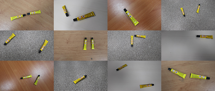
我将演示如何使用自定义数据集微调上述模型。为此，我创建了一个带有胶管的图像数据集，并为每个胶管（头部和尾部）分配了两个关键点。

1.图像和标注（自定义数据集）

该数据集包括 111 个训练图像和 23 个测试图像。每个图像都有一个或两个对象（胶管）。

每个图像的注释包括：

• 边界框坐标（每个物体都有一个边界框，用[x1, y1, x2, y2]格式即左上角和右下角坐标描述）；
• 关键点的坐标和可见性（每个对象有 2 个关键点，以 [x, y, visibility] 格式描述）。

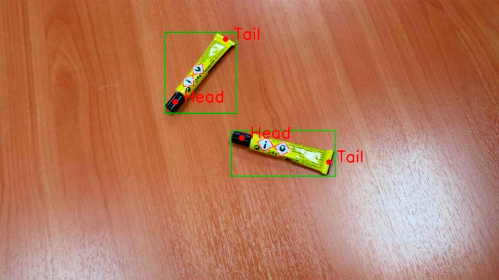
此数据集中的所有关键点都是可见的（即visibility=1）。第一个关键点是头部，第二个关键点是尾部。

你可以在这里下载数据集。

看看数据集中的几张随机图像和一张带有可视化标注的随机图像：

2.安装Pycocotools 库

在训练过程中，我们将评估我们模型的一些指标。这是在 pycocotools 库的帮助下完成的。继续并使用 pip install pycocotools 命令安装它。

为了评估预测的关键点与真实关键点的匹配程度，pycocotools 使用 COCOeval 类，默认情况下，该类被调整为评估人体的 17 个关键点。但是如果我们想要评估一组自定义的关键点（在我们的例子中它只有 2 个关键点），我们需要在该脚本中更改预定义的系数数组 kpt_oks_sigmas。

为此，我们需要打开 pycocotools/cocoeval.py 文件并更改行 self.kpt_oks_sigmas = np.array([.26, .25, .25, .35, .35, .79, .79, .72, .72, .62,.62, 1.07, 1.07, .87, .87, .89, .89])/10.0 到 self.kpt_oks_sigmas = np.array([.5, .5])/10.0

例如，在 Google Colab 中，可以通过以下路径找到该文件：/usr/local/lib/python3.7/dist-packages/pycocotools/cocoeval.py

您可以在此处阅读关键点评估指标、对象关键点相似度 (OKS) 和 OKS 系数的描述。

Update: 可以不编辑 pycocotools 库中的 pycocotools/cocoeval.py 文件来更改 kpt_oks_sigmas，而是编辑 coco_eval.py 文件：

# self.coco_eval[iou_type] = COCOeval(coco_gt, iouType=iou_type)
coco_eval = COCOeval(coco_gt, iouType=iou_type)
coco_eval.params.kpt_oks_sigmas = np.array([.5, .5]) / 10.0
self.coco_eval[iou_type] = coco_eval

3.代码实现

3.1 导入相关库

在 Jupyter Notebook 中创建一个新笔记本。首先，我们需要导入必要的模块：

import os, json, cv2, numpy as np, matplotlib.pyplot as plt

import torch
from torch.utils.data import Dataset, DataLoader

import torchvision
from torchvision.models.detection.rpn import AnchorGenerator
from torchvision.transforms import functional as F

import albumentations as A # Library for augmentations

接下来，从该存储库下载 coco_eval.py、coco_utils.py、engine.py、group_by_aspect_ratio.py、presets.py、train.py、transforms.py、utils.py 文件，并将它们放入笔记本所在的文件夹中。

也导入这些模块：

# https://github.com/pytorch/vision/tree/main/references/detection
import transforms, utils, engine, train
from utils import collate_fn
from engine import train_one_epoch, evaluate

3.2 数据增强

在这里，我们将为训练过程定义一个具有增强功能的函数。此函数将在每次训练迭代之前对图像应用不同的变换。在这些变换中，可以是亮度和对比度的随机变化，或图像旋转90度的随机次数。

因此，我们本质上是“创建新图像”，在某些方面与原始图像不同，但仍然非常适合训练我们的模型。

我们将使用almentations 库进行数据增强。

def train_transform():
    return A.Compose([
        A.Sequential([
            A.RandomRotate90(p=1), # Random rotation of an image by 90 degrees zero or more times
            A.RandomBrightnessContrast(brightness_limit=0.3, contrast_limit=0.3, brightness_by_max=True, always_apply=False, p=1), # Random change of brightness & contrast
        ], p=1)
    ],
    keypoint_params=A.KeypointParams(format='xy'), # More about keypoint formats used in albumentations library read at https://albumentations.ai/docs/getting_started/keypoints_augmentation/
    bbox_params=A.BboxParams(format='pascal_voc', label_fields=['bboxes_labels']) # Bboxes should have labels, read more at https://albumentations.ai/docs/getting_started/bounding_boxes_augmentation/
    )

3.3 Dataset 类

Dataset 类应该继承自标准的 torch.utils.data.Dataset 类，并且 __getitem__ 应该返回图像和targets。

以下是targets参数的说明：

• box (FloatTensor[N, 4])：[x0, y0, x1, y1] 格式的 N 个边界框的坐标。
• labels （Int64Tensor[N]）：每个边界框的标签。 0 始终代表背景类。
• image_id (Int64Tensor[1])：图像标识符。
• area (Tensor[N])：边界框的面积。
• iscrowd (UInt8Tensor[N]): iscrowd=True 的实例将在评估期间被忽略。
• keypoints (FloatTensor[N, K, 3])：对于 N 个对象中的每一个，它都包含 [x, y, visibility] 格式的 K 个关键点，定义对象。 visibility=0 表示关键点不可见。

让我们定义数据集类：

class ClassDataset(Dataset):
    def __init__(self, root, transform=None, demo=False):                
        self.root = root
        self.transform = transform
        self.demo = demo # Use demo=True if you need transformed and original images (for example, for visualization purposes)
        self.imgs_files = sorted(os.listdir(os.path.join(root, "images")))
        self.annotations_files = sorted(os.listdir(os.path.join(root, "annotations")))
    
    def __getitem__(self, idx):
        img_path = os.path.join(self.root, "images", self.imgs_files[idx])
        annotations_path = os.path.join(self.root, "annotations", self.annotations_files[idx])

        img_original = cv2.imread(img_path)
        img_original = cv2.cvtColor(img_original, cv2.COLOR_BGR2RGB)        
        
        with open(annotations_path) as f:
            data = json.load(f)
            bboxes_original = data['bboxes']
            keypoints_original = data['keypoints']
            
            # All objects are glue tubes
            bboxes_labels_original = ['Glue tube' for _ in bboxes_original]            

        if self.transform:   
            # Converting keypoints from [x,y,visibility]-format to [x, y]-format + Flattening nested list of keypoints            
            # For example, if we have the following list of keypoints for three objects (each object has two keypoints):
            # [[obj1_kp1, obj1_kp2], [obj2_kp1, obj2_kp2], [obj3_kp1, obj3_kp2]], where each keypoint is in [x, y]-format            
            # Then we need to convert it to the following list:
            # [obj1_kp1, obj1_kp2, obj2_kp1, obj2_kp2, obj3_kp1, obj3_kp2]
            keypoints_original_flattened = [el[0:2] for kp in keypoints_original for el in kp]
            
            # Apply augmentations
            transformed = self.transform(image=img_original, bboxes=bboxes_original, bboxes_labels=bboxes_labels_original, keypoints=keypoints_original_flattened)
            img = transformed['image']
            bboxes = transformed['bboxes']
            
            # Unflattening list transformed['keypoints']
            # For example, if we have the following list of keypoints for three objects (each object has two keypoints):
            # [obj1_kp1, obj1_kp2, obj2_kp1, obj2_kp2, obj3_kp1, obj3_kp2], where each keypoint is in [x, y]-format
            # Then we need to convert it to the following list:
            # [[obj1_kp1, obj1_kp2], [obj2_kp1, obj2_kp2], [obj3_kp1, obj3_kp2]]
            keypoints_transformed_unflattened = np.reshape(np.array(transformed['keypoints']), (-1,2,2)).tolist()

            # Converting transformed keypoints from [x, y]-format to [x,y,visibility]-format by appending original visibilities to transformed coordinates of keypoints
            keypoints = []
            for o_idx, obj in enumerate(keypoints_transformed_unflattened): # Iterating over objects
                obj_keypoints = []
                for k_idx, kp in enumerate(obj): # Iterating over keypoints in each object
                    # kp - coordinates of keypoint
                    # keypoints_original[o_idx][k_idx][2] - original visibility of keypoint
                    obj_keypoints.append(kp + [keypoints_original[o_idx][k_idx][2]])
                keypoints.append(obj_keypoints)
        
        else:
            img, bboxes, keypoints = img_original, bboxes_original, keypoints_original        
        
        # Convert everything into a torch tensor        
        bboxes = torch.as_tensor(bboxes, dtype=torch.float32)       
        target = {
    }
        target["boxes"] = bboxes
        target["labels"] = torch.as_tensor([1 for _ in bboxes], dtype=torch.int64) # all objects are glue tubes
        target["image_id"] = torch.tensor([idx])
        target["area"] = (bboxes[:, 3] - bboxes[:, 1]) * (bboxes[:, 2] - bboxes[:, 0])
        target["iscrowd"] = torch.zeros(len(bboxes), dtype=torch.int64)
        target["keypoints"] = torch.as_tensor(keypoints, dtype=torch.float32)        
        img = F.to_tensor(img)
        
        bboxes_original = torch.as_tensor(bboxes_original, dtype=torch.float32)
        target_original = {
    }
        target_original["boxes"] = bboxes_original
        target_original["labels"] = torch.as_tensor([1 for _ in bboxes_original], dtype=torch.int64) # all objects are glue tubes
        target_original["image_id"] = torch.tensor([idx])
        target_original["area"] = (bboxes_original[:, 3] - bboxes_original[:, 1]) * (bboxes_original[:, 2] - bboxes_original[:, 0])
        target_original["iscrowd"] = torch.zeros(len(bboxes_original), dtype=torch.int64)
        target_original["keypoints"] = torch.as_tensor(keypoints_original, dtype=torch.float32)        
        img_original = F.to_tensor(img_original)

        if self.demo:
            return img, target, img_original, target_original
        else:
            return img, target
    
    def __len__(self):
        return len(self.imgs_files)

以下是应用增强的数据集类部分的附加说明（紧跟在 if self.transform: 之后）：

Keypoint RCNN 的描述指出，关键点应以 [x, y, visibility] 格式提供。

如果我们想使用albumentations 库对图像及其标注应用数据增强功能，我们应该使用 [x, y] 格式。除此之外，所有关键点的列表不应嵌套。

因此，我们需要将初始列表中的关键点从[x, y, visibility]格式修改为[x, y]格式，并将列表平铺，然后应用数据增强，然后将列表恢复原状，并将关键点从[x, y]格式修改为[x, y, visibility]格式。

例如，如果图像包含两个对象，并且用列表 [[[392, 1247, 1], [152, 1055, 0]], [[530, 993, 1], [622, 660, 1]]]表示：

• 首先，我们将列表修改为 [[392, 1247], [152, 1055], [530, 993], [622, 660]]。
• 接下来，在我们应用了alphentations 增强之后，我们得到了一个转换后的关键点列表[[672, 392], [864, 152], [926, 530], [1259, 622]]。
• 最后，我们将转换后的关键点列表修改回 [[[672, 392, 1], [864, 152, 0]], [[926, 530, 1], [1259, 622, 1]]]。

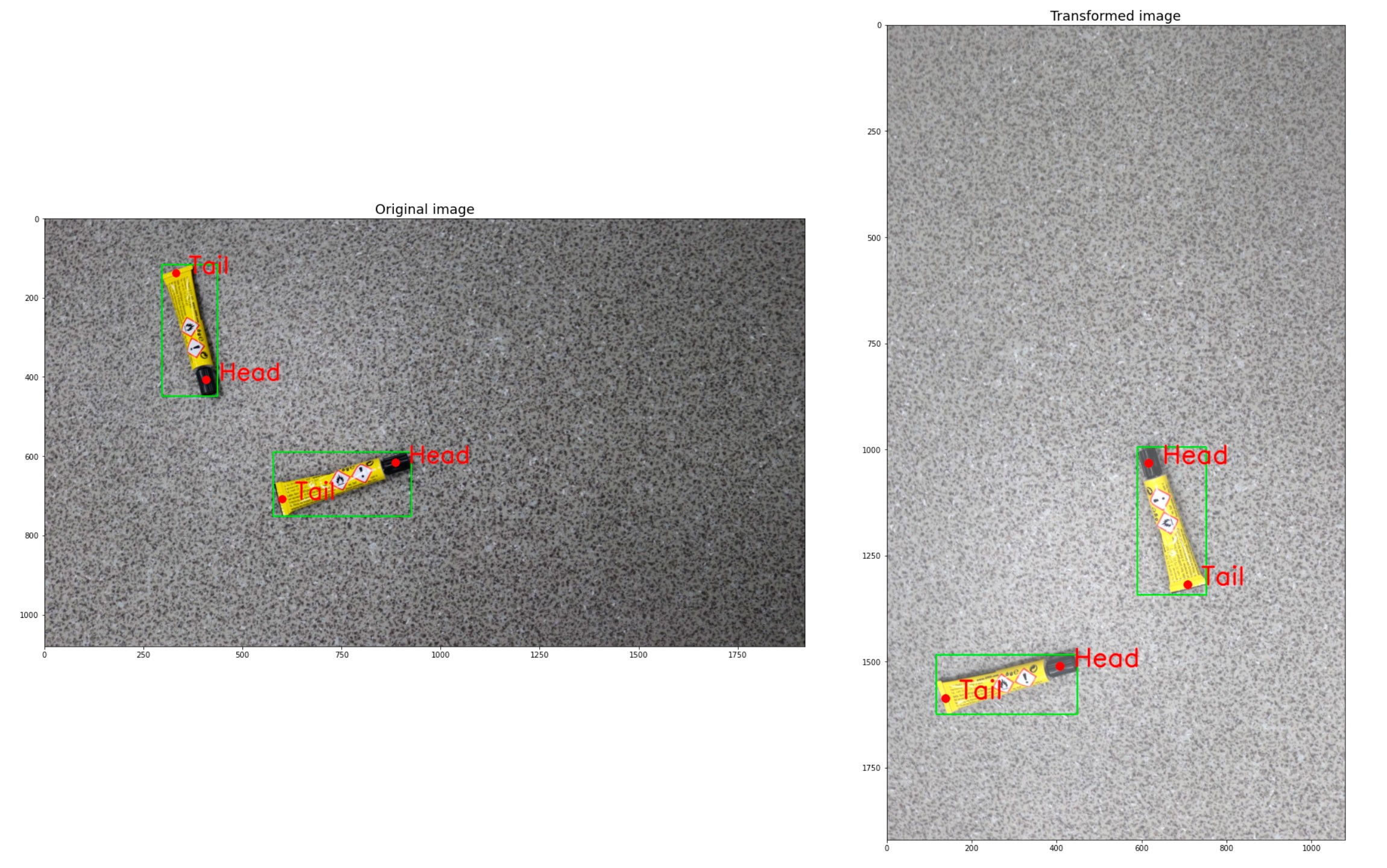
3.4 可视化数据集中的随机图像

KEYPOINTS_FOLDER_TRAIN = '/path/to/dataset/train'
dataset = ClassDataset(KEYPOINTS_FOLDER_TRAIN, transform=train_transform(), demo=True)
data_loader = DataLoader(dataset, batch_size=1, shuffle=True, collate_fn=collate_fn)

iterator = iter(data_loader)
batch = next(iterator)

print("Original targets:\n", batch[3], "\n\n")
print("Transformed targets:\n", batch[1])


# Original targets:
# ({'boxes': tensor([[296., 116., 436., 448.],
#                    [577., 589., 925., 751.]]),
# 'labels': tensor([1, 1]),
# 'image_id': tensor([15]),
# 'area': tensor([46480., 56376.]),
# 'iscrowd': tensor([0, 0]),
# 'keypoints': tensor([[[408., 407.,   1.],
#                       [332., 138.,   1.]],
#                      [[886., 616.,   1.],
#                       [600., 708.,   1.]]])},
# )
# Transformed targets:
# ({'boxes': tensor([[ 116., 1484.,  448., 1624.],
#                    [ 589.,  995.,  751., 1343.]]),
#   'labels': tensor([1, 1]),
#   'image_id': tensor([15]),
#   'area': tensor([46480., 56376.]),
#   'iscrowd': tensor([0, 0]),
#   'keypoints': tensor([[[4.0700e+02, 1.5110e+03, 1.0000e+00],
#                         [1.3800e+02, 1.5870e+03, 1.0000e+00]],
#                        [[6.1600e+02, 1.0330e+03, 1.0000e+00],
#                         [7.0800e+02, 1.3190e+03, 1.0000e+00]]])},
# )

在这里，我们将看一个原始图像和转换后图像的示例：

keypoints_classes_ids2names = {
    0: 'Head', 1: 'Tail'}

def visualize(image, bboxes, keypoints, image_original=None, bboxes_original=None, keypoints_original=None):
    fontsize = 18

    for bbox in bboxes:
        start_point = (bbox[0], bbox[1])
        end_point = (bbox[2], bbox[3])
        image = cv2.rectangle(image.copy(), start_point, end_point, (0,255,0), 2)
    
    for kps in keypoints:
        for idx, kp in enumerate(kps):
            image = cv2.circle(image.copy(), tuple(kp), 5, (255,0,0), 10)
            image = cv2.putText(image.copy(), " " + keypoints_classes_ids2names[idx], tuple(kp), cv2.FONT_HERSHEY_SIMPLEX, 2, (255,0,0), 3, cv2.LINE_AA)

    if image_original is None and keypoints_original is None:
        plt.figure(figsize=(40,40))
        plt.imshow(image)

    else:
        for bbox in bboxes_original:
            start_point = (bbox[0], bbox[1])
            end_point = (bbox[2], bbox[3])
            image_original = cv2.rectangle(image_original.copy(), start_point, end_point, (0,255,0), 2)
        
        for kps in keypoints_original:
            for idx, kp in enumerate(kps):
                image_original = cv2.circle(image_original, tuple(kp), 5, (255,0,0), 10)
                image_original = cv2.putText(image_original, " " + keypoints_classes_ids2names[idx], tuple(kp), cv2.FONT_HERSHEY_SIMPLEX, 2, (255,0,0), 3, cv2.LINE_AA)

        f, ax = plt.subplots(1, 2, figsize=(40, 20))

        ax[0].imshow(image_original)
        ax[0].set_title('Original image', fontsize=fontsize)

        ax[1].imshow(image)
        ax[1].set_title('Transformed image', fontsize=fontsize)
        
image = (batch[0][0].permute(1,2,0).numpy() * 255).astype(np.uint8)
bboxes = batch[1][0]['boxes'].detach().cpu().numpy().astype(np.int32).tolist()

keypoints = []
for kps in batch[1][0]['keypoints'].detach().cpu().numpy().astype(np.int32).tolist():
    keypoints.append([kp[:2] for kp in kps])

image_original = (batch[2][0].permute(1,2,0).numpy() * 255).astype(np.uint8)
bboxes_original = batch[3][0]['boxes'].detach().cpu().numpy().astype(np.int32).tolist()

keypoints_original = []
for kps in batch[3][0]['keypoints'].detach().cpu().numpy().astype(np.int32).tolist():
    keypoints_original.append([kp[:2] for kp in kps])

visualize(image, bboxes, keypoints, image_original, bboxes_original, keypoints_original)

3.5 训练

这里我们定义一个返回 Keypoint RCNN 模型的函数：

def get_model(num_keypoints, weights_path=None):
    
    anchor_generator = AnchorGenerator(sizes=(32, 64, 128, 256, 512), aspect_ratios=(0.25, 0.5, 0.75, 1.0, 2.0, 3.0, 4.0))
    model = torchvision.models.detection.keypointrcnn_resnet50_fpn(pretrained=False,
                                                                   pretrained_backbone=True,
                                                                   num_keypoints=num_keypoints,
                                                                   num_classes = 2, # Background is the first class, object is the second class
                                                                   rpn_anchor_generator=anchor_generator)

    if weights_path:
        state_dict = torch.load(weights_path)
        model.load_state_dict(state_dict)        
        
    return model

默认情况下，PyTorch 中的 AnchorGenerator 类有 3 种不同的尺寸 size=(128, 256, 512) 和 3 种不同的纵横比 aspect_ratios=(0.5, 1.0, 2.0) 看这里。我已经将这些参数扩展为 size=(32 , 64, 128, 256, 512) 和 aspect_ratios=(0.25, 0.5, 0.75, 1.0, 2.0, 3.0, 4.0)。

训练循环：

device = torch.device('cuda') if torch.cuda.is_available() else torch.device('cpu')

KEYPOINTS_FOLDER_TRAIN = '/path/to/dataset/train'
KEYPOINTS_FOLDER_TEST = '/path/to/dataset/test'

dataset_train = ClassDataset(KEYPOINTS_FOLDER_TRAIN, transform=train_transform(), demo=False)
dataset_test = ClassDataset(KEYPOINTS_FOLDER_TEST, transform=None, demo=False)

data_loader_train = DataLoader(dataset_train, batch_size=3, shuffle=True, collate_fn=collate_fn)
data_loader_test = DataLoader(dataset_test, batch_size=1, shuffle=False, collate_fn=collate_fn)

model = get_model(num_keypoints = 2)
model.to(device)

params = [p for p in model.parameters() if p.requires_grad]
optimizer = torch.optim.SGD(params, lr=0.001, momentum=0.9, weight_decay=0.0005)
lr_scheduler = torch.optim.lr_scheduler.StepLR(optimizer, step_size=5, gamma=0.3)
num_epochs = 5

for epoch in range(num_epochs):
    train_one_epoch(model, optimizer, data_loader_train, device, epoch, print_freq=1000)
    lr_scheduler.step()
    evaluate(model, data_loader_test, device)
    
# Save model weights after training
torch.save(model.state_dict(), '/path/to/folder/where/to/save/model/weights/keypointsrcnn_weights.pth')

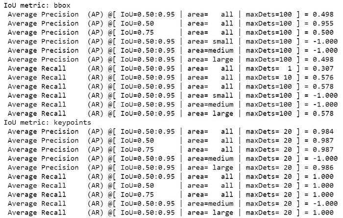
在训练循环中，我每批使用了 3 张图像。在这种情况下，使用了大约 10 GB 的 GPU VRAM，因此可以使用 Google Colab 训练模型。 在第 5 个 epoch 之后，我已经有了非常好的指标：

3.6 可视化模型预测

现在让我们看看经过训练的模型如何在测试数据集中的随机图像上预测胶管的边界框和关键点：

iterator = iter(data_loader_test)
images, targets = next(iterator)
images = list(image.to(device) for image in images)

with torch.no_grad():
    model.to(device)
    model.eval()
    output = model(images)

print("Predictions: \n", output)

输出

Predictions:
[{
    'boxes': tensor([[ 618.9335,  144.0377, 1111.2960,  529.3129],
                   [ 741.4827,  420.9630, 1244.8071,  930.4985],
                   [ 653.7405,  258.7889, 1018.7531,  509.9501],
                   [ 824.6623,  540.7152, 1170.4821,  886.6503],
                   [ 711.1497,    0.0000, 1134.0641, 1066.0247],
                   [ 708.5067,  177.0665, 1102.3306,  385.1994],
                   [ 657.0708,  398.0692,  987.9990,  498.4578],
                   [ 887.4133,  453.8322, 1184.2448,  727.9111],
                   [ 895.7014,   52.4423, 1106.8652, 1080.0000],
                   [ 545.8564,  318.9463, 1276.8043,  519.7277],
                   [ 732.6523,    0.0000,  891.0267,  918.9849],
                   [ 794.4460,  667.6695, 1091.6316,  861.5293],
                   [ 809.3927,  273.1192, 1037.3994,  915.0168],
                   [ 603.3748,  293.8343, 1473.1097,  860.4436],
                   [ 991.6447,  218.8240, 1144.5980,  924.2585],
                   [ 419.0262,  196.2676, 1204.9933,  679.9295],
                   [ 880.3656,  274.3975, 1166.3279,  863.6169],
                   [1006.1213,  478.2608, 1208.6801,  746.1869],
                   [ 390.1542,  234.1698, 1592.7747,  502.9070],
                   [ 433.5611,  472.5373, 1346.7277, 1010.1754],
                   [ 394.9036,   59.5816, 1268.1086,  491.0312]],                  device='cuda:0'),
  'labels': tensor([1, 1, 1, 1, 1, 1, 1, 1, 1, 1, 1, 1, 1, 1, 1, 1, 1, 1, 1, 1, 1], device='cuda:0'),
  'scores': tensor([0.9955, 0.9911, 0.7638, 0.7525, 0.7217, 0.3831, 0.3320, 0.3311, 0.2415, 0.1709, 0.1700, 0.1456, 0.1174, 0.1086, 0.1041, 0.1025, 0.0758, 0.0608, 0.0604, 0.0582, 0.0510], device='cuda:0'),
  'keypoints': tensor([[[6.6284e+02, 4.6822e+02, 1.0000e+00],
                        [1.0645e+03, 2.0082e+02, 1.0000e+00]],
  
                       [[1.1794e+03, 4.8645e+02, 1.0000e+00],
                        [8.3855e+02, 8.4773e+02, 1.0000e+00]],
  
                       [[6.6883e+02, 4.6905e+02, 1.0000e+00],
                        [6.5446e+02, 4.7048e+02, 1.0000e+00]],
  
                       [[8.2538e+02, 8.4989e+02, 1.0000e+00],
                        [8.4260e+02, 8.4557e+02, 1.0000e+00]],
  
                       [[1.1333e+03, 2.0672e+02, 1.0000e+00],
                        [8.3846e+02, 8.5642e+02, 1.0000e+00]],
  
                       [[1.0571e+03, 1.7778e+02, 1.0000e+00],
                        [1.0628e+03, 2.0219e+02, 1.0000e+00]],
  
                       [[6.7074e+02, 4.6476e+02, 1.0000e+00],
                        [6.5779e+02, 4.9774e+02, 1.0000e+00]],
  
                       [[1.1721e+03, 4.9329e+02, 1.0000e+00],
                        [1.1835e+03, 4.9329e+02, 1.0000e+00]],
  
                       [[1.1061e+03, 2.1457e+02, 1.0000e+00],
                        [1.0573e+03, 2.0160e+02, 1.0000e+00]],
  
                       [[6.6456e+02, 4.6882e+02, 1.0000e+00],
                        [6.6312e+02, 4.7025e+02, 1.0000e+00]],
  
                       [[8.9031e+02, 9.1682e+02, 1.0000e+00],
                        [8.4279e+02, 8.5057e+02, 1.0000e+00]],
  
                       [[7.9516e+02, 8.6081e+02, 1.0000e+00],
                        [8.3823e+02, 8.4358e+02, 1.0000e+00]],
  
                       [[8.1011e+02, 8.4521e+02, 1.0000e+00],
                        [8.4166e+02, 8.4809e+02, 1.0000e+00]],
  
                       [[6.6745e+02, 4.6612e+02, 1.0000e+00],
                        [8.3017e+02, 8.5828e+02, 1.0000e+00]],
  
                       [[1.1439e+03, 4.9884e+02, 1.0000e+00],
                        [1.0696e+03, 2.2098e+02, 1.0000e+00]],
  
                       [[6.6590e+02, 4.6905e+02, 1.0000e+00],
                        [1.0632e+03, 1.9699e+02, 1.0000e+00]],
  
                       [[1.1656e+03, 4.9553e+02, 1.0000e+00],
                        [8.8108e+02, 8.6146e+02, 1.0000e+00]],
  
                       [[1.1749e+03, 4.9195e+02, 1.0000e+00],
                        [1.1749e+03, 4.7898e+02, 1.0000e+00]],
  
                       [[6.6741e+02, 4.6914e+02, 1.0000e+00],
                        [1.1859e+03, 5.0219e+02, 1.0000e+00]],
  
                       [[1.1804e+03, 4.7470e+02, 1.0000e+00],
                        [8.3901e+02, 8.4514e+02, 1.0000e+00]],
  
                       [[6.6463e+02, 4.9031e+02, 1.0000e+00],
                       [1.0646e+03, 1.9980e+02, 1.0000e+00]]],  device='cuda:0'),
  'keypoints_scores': tensor([[36.9580, 26.7403],
                              [31.9451, 28.6134],
                              [22.5176, -0.4728],
                              [ 7.7444, 21.3082],
                              [ 1.3215,  7.6223],
                              [ 2.0522, 22.6735],
                              [26.5938, -2.3956],
                              [19.8818,  2.7854],
                              [ 0.5259, 16.2155],
                              [39.5929, -0.1582],
                              [ 0.4924, 21.0935],
                              [ 0.5597, 19.3637],
                              [ 3.4223, 25.5078],
                              [17.6618,  0.4896],
                              [ 5.9306, -1.5709],
                              [27.4080,  2.4160],
                              [11.7086, -1.3879],
                              [26.0192,  3.0886],
                              [15.6420, -1.7428],
                              [ 7.1422, 10.9291],
                              [14.1688, 15.1565]], device='cuda:0')}]

在这里，我们看到了很多预测对象。我们将只选择置信度得分高的那些（例如，> 0.7）。然后我们将应用非最大抑制（NMS）程序在剩余的边界框中选择最合适的边界框。

本质上，NMS 会留下置信度得分最高的框（最佳候选者）并移除与最佳候选者部分重叠的其他框。为了定义这种重叠的程度，我们将 Intersection over Union (IoU) 的阈值设置为 0.3。

在PyTorch中阅读更多关于NMS实现的信息。

让我们可视化预测：

image = (images[0].permute(1,2,0).detach().cpu().numpy() * 255).astype(np.uint8)
scores = output[0]['scores'].detach().cpu().numpy()

high_scores_idxs = np.where(scores > 0.7)[0].tolist() # Indexes of boxes with scores > 0.7
post_nms_idxs = torchvision.ops.nms(output[0]['boxes'][high_scores_idxs], output[0]['scores'][high_scores_idxs], 0.3).cpu().numpy() # Indexes of boxes left after applying NMS (iou_threshold=0.3)

# Below, in output[0]['keypoints'][high_scores_idxs][post_nms_idxs] and output[0]['boxes'][high_scores_idxs][post_nms_idxs]
# Firstly, we choose only those objects, which have score above predefined threshold. This is done with choosing elements with [high_scores_idxs] indexes
# Secondly, we choose only those objects, which are left after NMS is applied. This is done with choosing elements with [post_nms_idxs] indexes

keypoints = []
for kps in output[0]['keypoints'][high_scores_idxs][post_nms_idxs].detach().cpu().numpy():
    keypoints.append([list(map(int, kp[:2])) for kp in kps])

bboxes = []
for bbox in output[0]['boxes'][high_scores_idxs][post_nms_idxs].detach().cpu().numpy():
    bboxes.append(list(map(int, bbox.tolist())))
    
visualize(image, bboxes, keypoints)

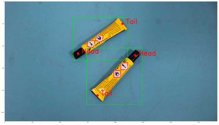
预测看起来不错：边界框几乎是精确的，关键点在正确的位置。这意味着模型训练得很好。 以同样的方式，您可以使用另一个数据集训练 Keypoint RCNN，选择任意数量的关键点。

这是一个包含上述所有步骤的 GitHub 存储库和笔记本。

参考目录

https://medium.com/@alexppppp/how-to-train-a-custom-keypoint-detection-model-with-pytorch-d9af90e111da